Multivariate statistics

The purpose of this vignette is to demonstrate how we can use the MultivariateStats package on layers.

This functionality is supported through an extension, which is only active when the MultivariateStats package is loaded.

julia

using SpeciesDistributionToolkit
using CairoMakie
using Statistics
import StatsBase
using MultivariateStats

The support is currently limited to PCA

julia

spatial_extent = (left = 8.412, bottom = 41.325, right = 9.662, top = 43.060)
dataprovider = RasterData(CHELSA1, BioClim)
L = [SDMLayer(dataprovider; layer = i, spatial_extent...) for i in [1, 3, 8, 12]]

4-element Vector{SDMLayer{Int16}}:
 🗺️  A 209 × 151 layer (14432 Int16 cells)
 🗺️  A 209 × 151 layer (14432 Int16 cells)
 🗺️  A 209 × 151 layer (14432 Int16 cells)
 🗺️  A 209 × 151 layer (14432 Int16 cells)

We can fit a PCA the "normal" way:

julia

M = fit(PCA, L; maxoutdim=2)

PCA(indim = 4, outdim = 2, principalratio = 0.9861689593337618)

Pattern matrix (unstandardized loadings):
──────────────────────
        PC1        PC2
──────────────────────
1  -25.3517  17.6834
2   10.803   -0.856928
3  -28.2572  23.5815
4  153.092    7.34138
──────────────────────

Importance of components:
────────────────────────────────────────────────────
                                    PC1          PC2
────────────────────────────────────────────────────
SS Loadings (Eigenvalues)  24995.0       923.419
Variance explained             0.951034    0.0351351
Cumulative variance            0.951034    0.986169
Proportion explained           0.964372    0.0356279
Cumulative proportion          0.964372    1.0
────────────────────────────────────────────────────

Note that this will return a PCA result object. We can use it to project a vector of layers:

julia

X = predict(M, L)

2-element Vector{SDMLayer{Float64}}:
 🗺️  A 209 × 151 layer (14432 Float64 cells)
 🗺️  A 209 × 151 layer (14432 Float64 cells)

The last argument must be a vector of layers (or a vector of layers), which will be used as a template to store the output values in.

Data leakage

Transforming the layers before extracting the values of environmental conditions for SDMs creates data leakage and should never be done. SDeMo handles projections the correct way.

We can visualize the result of this projection (first principal component):

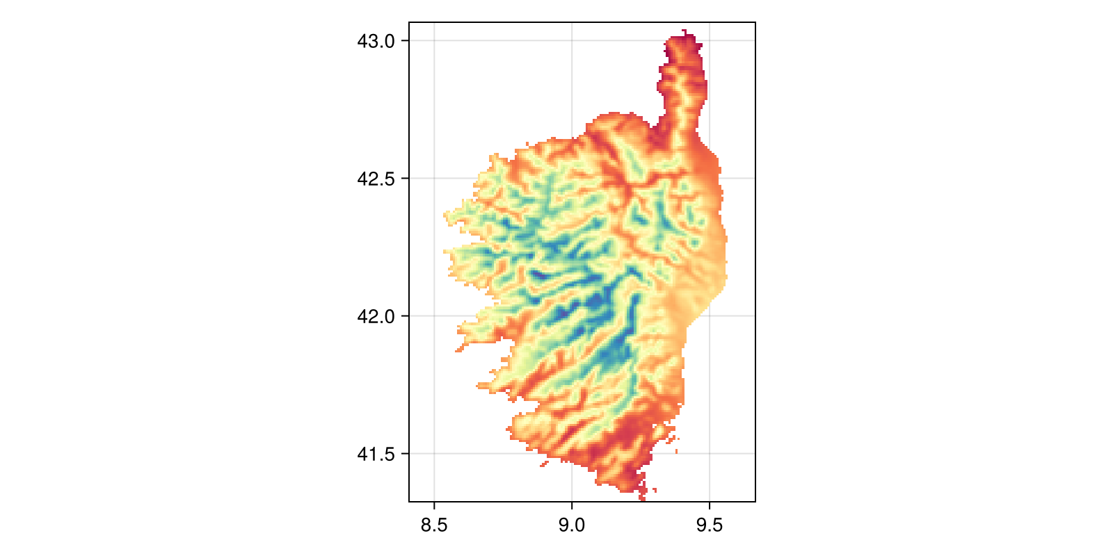
Code for the figure

julia

fig, ax, hm = heatmap(
    X[1],
    colormap = :Spectral,
    figure = (; size = (800, 400)),
    axis = (; aspect = DataAspect()),
)

Multivariate statistics ​

Multivariate statistics