Zonal statistics

In this tutorial, we will grab some bioclimatic variables for Bretagne, and then identify the departments that have extreme values of this variable.

using SpeciesDistributionToolkit
using Statistics
using CairoMakie

We can get polygon data from Open Street Map:

BZH = SpeciesDistributionToolkit.openstreetmap("Bretagne")
departements = ["Ille-et-Vilaine", "Morbihan", "Côtes-d'Armor", "Finistère"]
DPTs = SpeciesDistributionToolkit.openstreetmap.(departements)

4-element Vector{GeoJSON.MultiPolygon{2, Float32}}:
 2D MultiPolygonwith 47 sub-geometries
 2D MultiPolygonwith 198 sub-geometries
 2D MultiPolygonwith 312 sub-geometries
 2D MultiPolygonwith 827 sub-geometries

We will get the BIO1 layer from CHELSA2 (average annual temperature):

spatial_extent = SpeciesDistributionToolkit.boundingbox(BZH; padding = 0.2)
dataprovider = RasterData(CHELSA2, BioClim)
layer = SDMLayer(dataprovider; layer = "BIO1", spatial_extent...)

🗺️  A 269 × 545 layer with 146605 UInt16 cells
   Projection: +proj=longlat +datum=WGS84 +no_defs

This layer is trimmed to the landmass (according to GADM):

mask!(layer, BZH)
layer = trim(layer)

🗺️  A 220 × 494 layer with 47858 UInt16 cells
   Projection: +proj=longlat +datum=WGS84 +no_defs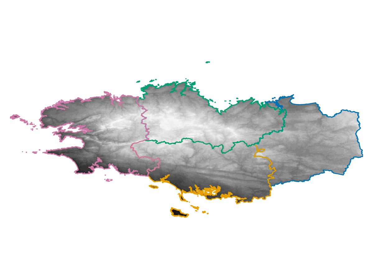

Code for the figure

fig, ax, plt = heatmap(layer; axis = (; aspect = DataAspect()), colormap = :Greys)
hidespines!(ax)
hidedecorations!(ax)
lines!.(DPTs)

We can start looking at how the departments map onto the landscape, using the zone function. It will return a layer where the value of each pixel is the index of the polygon containing this pixel:

Code for the figure

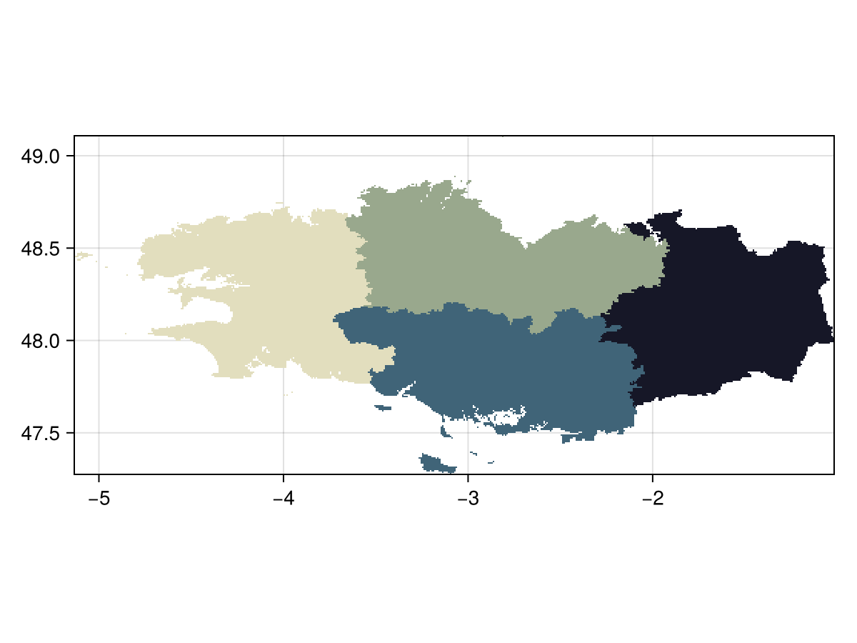
heatmap(zone(layer, DPTs); colormap = :hokusai, axis = (; aspect = DataAspect()))

Note that the pixels that are not within a polygon are turned off, which can sometimes happen if the overlap between polygons is not perfect. There is a variant of the mosaic method that uses polygon to assign the values:

z = mosaic(mean, layer, DPTs)
nodata!(z, 0.0)

🗺️  A 220 × 494 layer with 47858 Float64 cells
   Projection: +proj=longlat +datum=WGS84 +no_defs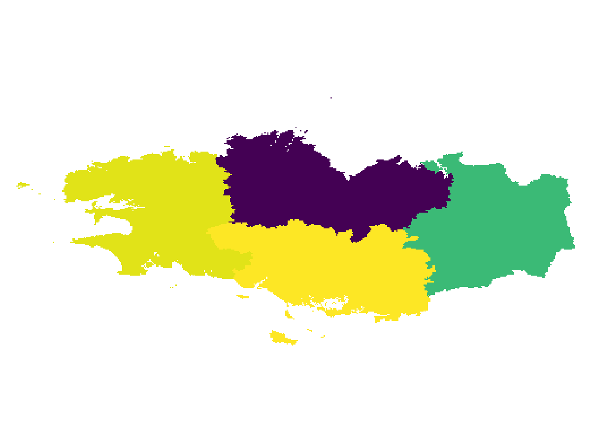

Code for the figure

fig, ax, plt = heatmap(z; axis = (; aspect = DataAspect()))
hidespines!(ax)
hidedecorations!(ax)

Finally, we can get the mean value within each of these polygons using the byzone method:

depts_ranked = sort(
    byzone(mean, layer, DPTs, departements);
    by = (x) -> x.second,
    rev = true,
)

4-element Vector{Pair{String, Float64}}:
        "Morbihan" => 2847.1600807129644
       "Finistère" => 2846.9205745669624
 "Ille-et-Vilaine" => 2845.4547211021504
   "Côtes-d'Armor" => 2841.8226584867075

The index of the department with the highets value is

i = findfirst(isequal(depts_ranked[1].first), departements)

2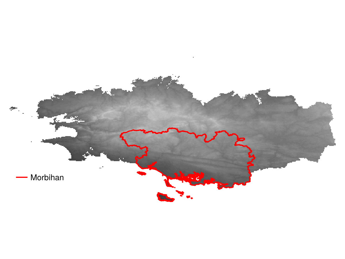

Code for the figure

fig, ax, plt =
    heatmap(layer; axis = (; aspect = DataAspect()), colormap = [:grey80, :grey20])
lines!(ax, DPTs[i]; label = departements[i], linewidth = 2, color=:red)
axislegend(; position = (0, 0.1), nbanks = 1, framevisible=false)