Variograms

The package has limited functionalities to generate and fit empirical variograms. These are intended as companion functions to the tessellation feature, in order to approximate a relevant size for the tiling.

Unstable part of the API

The functions on this page should be considered a work in progress, and their behavior is likely to change in ways that will be documented here. These should be treated primarily as convenience functions.

using SpeciesDistributionToolkit
const SDT = SpeciesDistributionToolkit
using PrettyTables
using CairoMakie

using Statistics

Variograms on layers

We will start by grabbing some information on temperature over the island of Corsica.

polygon = getpolygon(PolygonData(OpenStreetMap, Places); place = "Corse")
temperature = SDMLayer(RasterData(CHELSA2, AverageTemperature); SDT.boundingbox(polygon)...)
mask!(temperature, polygon);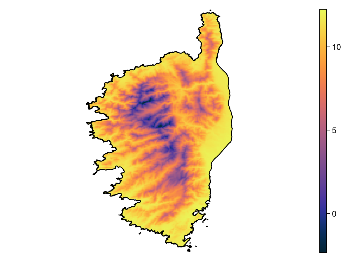

Code for the figure

f = Figure()
ax = Axis(f[1, 1]; aspect = DataAspect())
hm = heatmap!(ax, temperature; colormap = :thermal)
lines!(ax, polygon; color = :black)
hidespines!(ax)
hidedecorations!(ax)
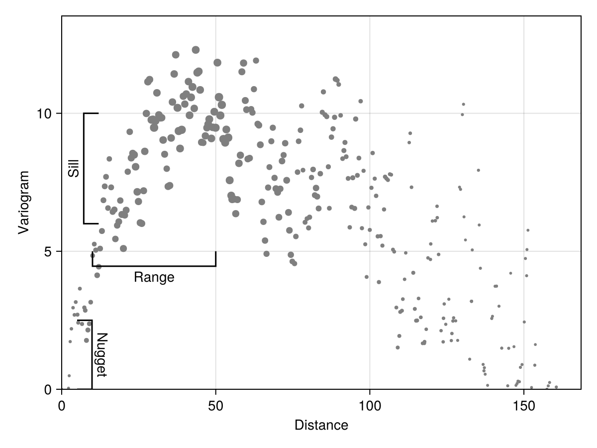
Colorbar(f[1, 2], hm)

To measure the empirical semi-variogram from this dataset, we need to specify the width of each bin, and by how much each bin is shifted from one to the other. The variogram function will guesstimate the number of point pairs to measure in order to ensure that the average coverage of each bin is around 30 samples.

x, y, n = variogram(temperature; width = 2.0, shift = 0.5);

The variogram function will return the average distance within the bin x, the variance within this bin y, and the number of point pairs used to generate this bin n. This last information is important to fit a variogram model (as we will discuss later).

Code for the figure

f = Figure()
ax = Axis(f[1, 1]; xlabel = "Distance", ylabel = "Variogram")
scatter!(ax, x, y; markersize = n ./ maximum(n) .* 8 .+ 4, color = :grey50)
bracket!(ax, 10., 5., 50., 5., text="Range", style=:square, orientation=:down)
bracket!(ax, 5., 0., 5., 2.5, text="Nugget", style=:square, orientation=:down)
bracket!(ax, 12., 6., 12., 10., text="Sill", style=:square, orientation=:up)
ylims!(ax, 0.0, 1.1*maximum(y))
xlims!(ax; low = 0.0)

Note that the values end up being very correlated at extremely high distances, which makes sense: the climate is similar everywhere on the coasts, and some of the furthest points (in space) are therefore the most similar.

Fitting a model to the variogram

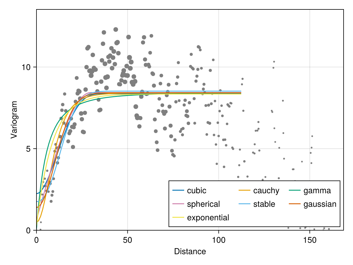
The unexported fitvariogram method will get the parameters for one of the usual variogram models (there are other models, see the documentation for this function):

families = [:gaussian, :spherical, :exponential, :cubic, :stable, :cauchy, :gamma]

7-element Vector{Symbol}:
 :gaussian
 :spherical
 :exponential
 :cubic
 :stable
 :cauchy
 :gamma

In order to ensure that the parameters make sense, we will look at the previously generated figure and come up with an estimated range for the parameters. These parameters correspond to the annotated rangebars on the previous figure.

params = (;
    sill = (6.0, 10.0),
    nugget = (0.0, 2.5),
    range = (10.0, 50.0),
    parameter = (0.05, 2.5),
)

(sill = (6.0, 10.0), nugget = (0.0, 2.5), range = (10.0, 50.0), parameter = (0.05, 2.5))

The parameter is not used by all methods, but is required to be estimated for :gamma, :cauchy, and :stable. Note that :hyperbolic is a specific case of :gamma with the parameter fixed to 1.

We will collect all these models in a dictionary. To gain time, this is multi-threaded:

fits = map(families) do family
    Threads.@spawn begin
        return family => SDT.fitvariogram(x, y, n; family = family, params...)
    end
end
M = fetch.(fits)
D = Dict(M);

This function relies on the Nelder-Mead solver to find an approximate value of the parameters. Note that the error associated to each parameter set accounts for the number of samples in each bin, and that samples get linearly less weight with decreasing number of observations.

The outputs are named tuples with fields for the nugget, sill, range, as well as the error, and a function giving the best model.

Code for the figure

f = Figure()
ax = Axis(f[1, 1]; xlabel = "Distance", ylabel = "Variogram")
scatter!(ax, x, y; markersize = n ./ maximum(n) .* 8 .+ 4, color = :grey50)
vx = LinRange(0.0, 0.7 * maximum(x), 100)
for (fam, mod) in D
    lines!(ax, vx, mod.model.(vx); label = string(fam))
end
ylims!(ax, 0.0, 1.1*maximum(y))
xlims!(ax; low = 0.0)
axislegend(ax; position = :rb, nbanks = 3)

We can aggregate this information to figure out which model describes the data better:

M = permutedims(
    hcat([[fam, mod.range, mod.nugget, mod.sill, mod.error] for (fam, mod) in D]...),
)
rnk = sortperm(M[:, 5])
M = M[rnk, :];

pretty_table(
    M;
    alignment = [:l, :c, :c, :c, :c],
    backend = :markdown,
    column_labels = ["Model", "Range", "Nugget", "Sill", "RMSE"],
    formatters = [
        fmt__printf("%5.2f", [2, 3, 4]),
        fmt__printf("%7.4f", [5]),
    ],
)

Model	Range	Nugget	Sill	RMSE
spherical	29.72	0.65	8.43	2.1323
gaussian	24.80	1.39	8.42	2.1361
cubic	38.25	2.24	8.37	2.1376
stable	26.46	1.75	8.52	2.1423
cauchy	24.99	0.49	8.43	2.1572
exponential	26.34	0.29	8.34	2.1913
gamma	33.31	0.08	8.46	2.2539

Variogram on SDMs

Variograms can also be generated on the training data of an SDM. We will grab enough data to train an SDM:

L = [
    SDMLayer(RasterData(CHELSA2, BioClim); SDT.boundingbox(polygon)..., layer = i) for
    i in 1:19
]
mask!(L, polygon)
records = SDeMo.__demodata()
model = SDM(RawData, Logistic, records...)
variables!(model, ForwardSelection)

☑️  RawData → Logistic → P(x) ≥ 0.543 🗺️

To generate the variogram from these data, we need to specify a variable through the keywword argument of the same name:

x, y, n = variogram(model; variable = 1, width = 2.0, shift = 1.0);
sdm_vario = SDT.fitvariogram(x, y, n; family = :spherical);

We will also compare this to the variogram that would have been obtained on the layer:

xl, yl, nl = variogram(L[1]; width = 2.0, shift = 1.0);
layer_vario = SDT.fitvariogram(xl, yl, nl; family = :spherical);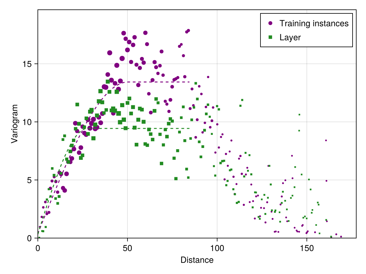

Code for the figure

f = Figure()
ax = Axis(f[1, 1]; xlabel = "Distance", ylabel = "Variogram")
vx = LinRange(0.0, maximum(x) / 2, 100)
scatter!(
    ax,
    x,
    y;
    markersize = n ./ maximum(n) .* 8 .+ 4,
    color = :purple,
    label = "Training instances",
)
lines!(ax, vx, sdm_vario.model.(vx); color = :purple, linestyle = :dash)
scatter!(
    ax,
    xl,
    yl;
    markersize = nl ./ maximum(nl) .* 8 .+ 4,
    color = :forestgreen,
    marker = :rect,
    label = "Layer",
)
lines!(ax, vx, layer_vario.model.(vx); color = :forestgreen, linestyle = :dash)
axislegend(ax; position = :rt)
ylims!(ax, 0.0, 1.1*maximum(y))
xlims!(ax; low = 0.0)

We can measure the range that corresponds to the variation of each variable selected by the model:

variomodels = [
    SDT.fitvariogram(variogram(model; variable = i)...; family = :spherical)
    for i in variables(model)
];
ranges = [m.range for m in variomodels]

7-element Vector{Float64}:
  61.768536597051906
  93.8662022479391
  85.11655390014404
  82.93769862028873
  89.14994049534573
 107.62692462907644
  47.534954240702795

We can then, for example, get the median range across all these variables, which is a common approximation for the correct block size to use in spatial cross-validation.

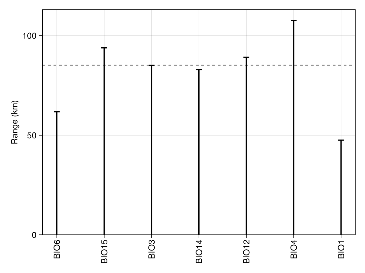
Code for the figure

f = Figure()
xticks = (
    1:length(variables(model)),
    "BIO" .* string.(variables(model)),
)
ax = Axis(f[1, 1]; ylabel = "Range (km)", xticks = xticks, xticklabelrotation = π / 2)
hlines!(ax, [median(ranges)]; color = :grey50, linestyle = :dash)
stem!(
    ax,
    ranges;
    trunkcolor = :transparent,
    color = :black,
    stemcolor = :black,
    stemwidth = 2,
    markersize = 15,
    marker = :hline,
)
ylims!(ax; low = 0.0)

Variogram on occurrences

We can also generate the variogram on a collection of occurrences, which is primarily useful to check the distance at which two observations are likely to be different.

x, y, n = variogram(Occurrences(model), width = 2.0, shift = 1.0);
occ_vario = SDT.fitvariogram(
    x, y, n;
    family = :stable
);

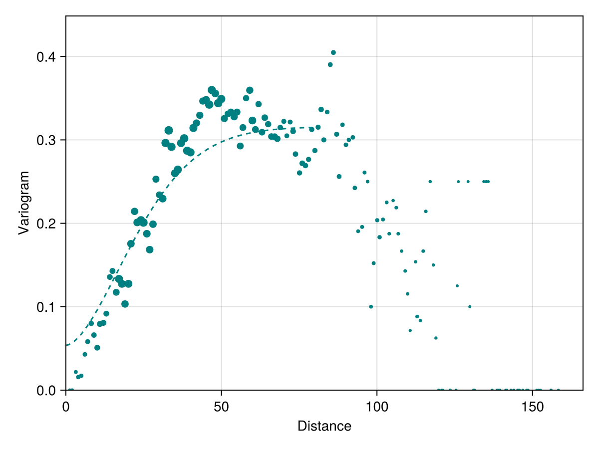
Code for the figure

f = Figure()
vx = LinRange(0.0, maximum(x) * 0.5, 100)
ax = Axis(f[1, 1]; xlabel = "Distance", ylabel = "Variogram")
scatter!(ax, x, y; markersize = n ./ maximum(n) .* 8 .+ 4, color = :teal)
lines!(ax, vx, occ_vario.model.(vx); color = :teal, linestyle = :dash)
ylims!(ax, 0.0, only(quantile(y, [0.99])))
xlims!(ax; low = 0.0)

Related documentation

SpeciesDistributionToolkit.variogram Function

variogram(L::SDMLayer; samples::Integer=2000, bins::Integer=100; kwargs...)

Generates the raw data to look at an empirical semivariogram from a layer with numerical values. This method will generate bins that are width kilometers wide by drawing pairs of points at random, and each bin will be shifted by shift kilometers.

This returns three vectors: the empirical center of the bin, the semivariance within this bin, and the number of samples that compose this bin.

source

variogram(model::AbstractSDM; variable::Int, samples::Integer=2000, bins::Integer=100; kwargs...)

Generates the raw data to look at an empirical semivariogram from a model, for a given variable (keyword, defaults to the first variable in the model). This method will generate bins that are width kilometers wide by drawing pairs of points at random, and each bin will be shifted by shift kilometers.

This returns three vectors: the empirical center of the bin, the semivariance within this bin, and the number of samples that compose this bin.

source

variogram(occ::AbstractOccurrenceCollection; width::Float64 = 10., shift::Float64=1.0, kwargs...)

Generates the raw data to look at an empirical semivariogram from a collection of occurrences. This method will generate bins that are width kilometers wide by drawing pairs of points at random, and each bin will be shifted by shift kilometers.

This returns three vectors: the empirical center of the bin, the semivariance within this bin, and the number of samples that compose this bin.

source

SpeciesDistributionToolkit.fitvariogram Function

fitvariogram(x, y, n; family = :gaussian)

Fits a variogram of the given family based on data representing the central bin distance x, the semivariogram y, and the sample size n. The data are returned as a named tuple containing the range, the sill, the nugget, the parameter, the error (RMSE), and the model. The model is a function that can be called on a given distance to obtain the best fit variogram (see the details below).

The family keyword (defaults to :gaussian) selects the type of variogram model to fit. Families of :gaussian, :spherical, :exponential, :linear, :cubic, and :hyperbolic only fit the range, nugget, and sill. Families of :gamma, :stable, :cauchy also fit a free parameter. Finally, :cardinalsine can be used to fit periodic variograms.

Values are optimized using the Nelder-Mead algorithm with samples samples (300) and maxiter iterations (1200). The tol criteria (10⁻⁴) is the threshold under which the variance of the RMSE is assumed to indicate that the algorithm has converged and should return early. After the algorithm has concluded, the best candidate parameter set is returned.

To help the optimisation process, it is a good idea to provide some guidance to the algorithm in the form of boundaries for the various parameters, as tuple of floats. By default, the range boundary is from the shortest distance to 3/4th of the maximum distance; the sill is within the extrema of the observed variances; the nugget boundary is between the smallest variance observed and half of the max; the parameter boundary is between 0.1 and 2. Visual inspection of the empirical data will help set realistic values.

source

fitvariogram(L::SDMLayer; family::Symbol=:gaussian, kwargs...)

Fits the variogram based on a layer. The kwargs... are passed to variogram.

source