Use with the SDeMo package

In this tutorial, we will see how to deal with ensemble models. It is assumed that you will have read the previous tutorial, explaining how to use prediction functions more generally.

using SpeciesDistributionToolkit
using CairoMakie
using Statistics
using Dates

Getting the data

CHE = SpeciesDistributionToolkit.openstreetmap("Switzerland");

We get the data on the BioClim variables from CHELSA2:

provider = RasterData(CHELSA2, BioClim)
L = SDMLayer{Float32}[
    SDMLayer(
        provider;
        layer = x,
        SpeciesDistributionToolkit.boundingbox(CHE)...,
    ) for x in 1:19
];

And we then clip and trim to the polygon describing Switzerland:

L = mask!(L, CHE)

19-element Vector{SDMLayer{Float32}}:
 🗺️  A 240 × 546 layer (70065 Float32 cells)
 🗺️  A 240 × 546 layer (70065 Float32 cells)
 🗺️  A 240 × 546 layer (70065 Float32 cells)
 🗺️  A 240 × 546 layer (70065 Float32 cells)
 🗺️  A 240 × 546 layer (70065 Float32 cells)
 🗺️  A 240 × 546 layer (70065 Float32 cells)
 🗺️  A 240 × 546 layer (70065 Float32 cells)
 🗺️  A 240 × 546 layer (70065 Float32 cells)
 🗺️  A 240 × 546 layer (70065 Float32 cells)
 🗺️  A 240 × 546 layer (70065 Float32 cells)
 🗺️  A 240 × 546 layer (70065 Float32 cells)
 🗺️  A 240 × 546 layer (70065 Float32 cells)
 🗺️  A 240 × 546 layer (70065 Float32 cells)
 🗺️  A 240 × 546 layer (70065 Float32 cells)
 🗺️  A 240 × 546 layer (70065 Float32 cells)
 🗺️  A 240 × 546 layer (70065 Float32 cells)
 🗺️  A 240 × 546 layer (70065 Float32 cells)
 🗺️  A 240 × 546 layer (70065 Float32 cells)
 🗺️  A 240 × 546 layer (70065 Float32 cells)

The next step is to get the data, using the eBird dataset:

ouzel = taxon("Turdus torquatus")
presences = occurrences(
    ouzel,
    first(L),
    "occurrenceStatus" => "PRESENT",
    "limit" => 300,
    "datasetKey" => "4fa7b334-ce0d-4e88-aaae-2e0c138d049e",
)
while length(presences) < count(presences)
    occurrences!(presences)
end

And after this, we prepare a layer with presence data.

presencelayer = mask(first(L), Occurrences(mask(presences, CHE)))

🗺️  A 240 × 546 layer with 70065 Bool cells
   Projection: +proj=longlat +datum=WGS84 +no_defs

The next step is to generate a pseudo-absence mask. There is a longer explanation on the ways to generate pseudo-absences in the "How-to" section of the manual. We will sample based on the distance to an observation, by also preventing pseudo-absences to be less than 4km from an observation:

background = pseudoabsencemask(DistanceToEvent, presencelayer)
bgpoints = backgroundpoints(nodata(background, d -> d < 4), 2sum(presencelayer))

🗺️  A 240 × 546 layer with 45362 Bool cells
   Projection: +proj=longlat +datum=WGS84 +no_defs

Setting up the model

We will use a decision tree on data transformed through a PCA. Because we will eventually use an ensemble, we want the trees to be shallow (but not too shallow):

sdm = SDM(PCATransform, DecisionTree, L, presencelayer, bgpoints)
variables!(sdm, ForwardSelection, kfold(sdm))

PCATransform → DecisionTree → P(x) ≥ 0.458

Making the first prediction

We can predict using the model by giving a vector of layers as an input. This will return the output as a layer as well:

prd = predict(sdm, L; threshold = false)

🗺️  A 240 × 546 layer with 70065 Float64 cells
   Projection: +proj=longlat +datum=WGS84 +no_defs

This gives the following initial prediction:

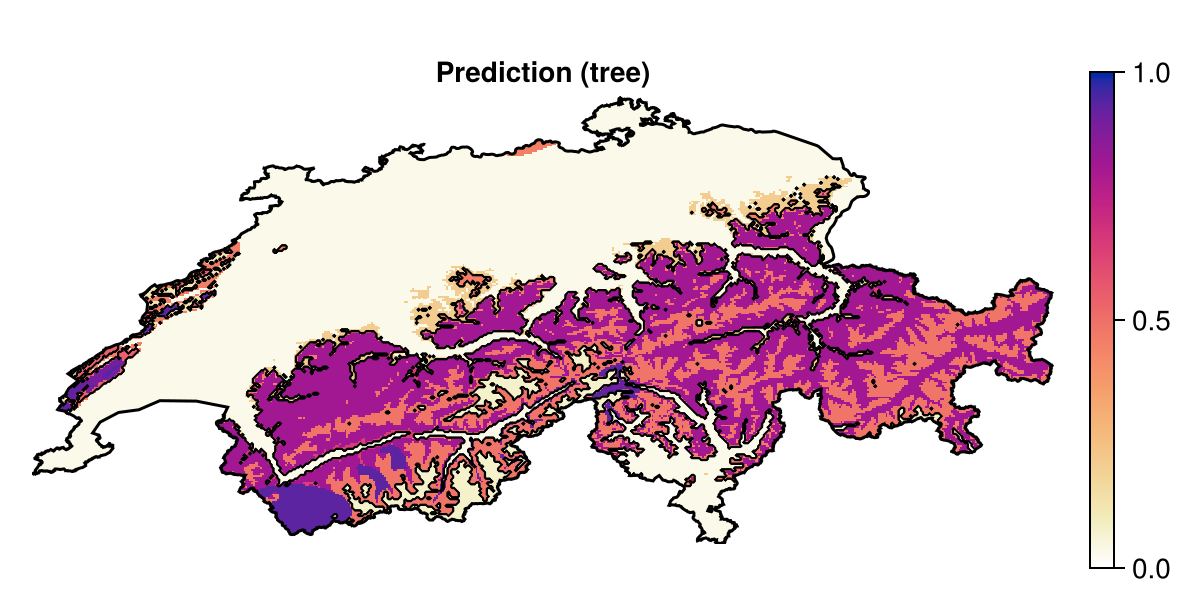
Code for the figure

f = Figure(; size = (600, 300))
ax = Axis(f[1, 1]; aspect = DataAspect(), title = "Prediction (tree)")
hm = heatmap!(ax, prd; colormap = :linear_worb_100_25_c53_n256, colorrange = (0, 1))
contour!(ax, predict(sdm, L); color = :black, linewidth = 0.5)
Colorbar(f[1, 2], hm)
lines!(ax, CHE; color = :black)
hidedecorations!(ax)
hidespines!(ax)

We can now create an ensemble model, by boostrapping random instances to train a larger number of trees:

ensemble = Bagging(sdm, 30)

{PCATransform → DecisionTree → P(x) ≥ 0.458} × 30

In order to further ensure that the models are learning from different parts of the dataset, we can also bootstrap which variables are accessible to each model:

bagfeatures!(ensemble)

{PCATransform → DecisionTree → P(x) ≥ 0.458} × 30

By default, the bagfeatures! function called on an ensemble will sample the variables forom the model, so that each model in the ensemble has the square root (rounded up) of the number of original variables.

A probably better alternative is to reset the variables of our model:

variables!(ensemble, AllVariables)

{PCATransform → DecisionTree → P(x) ≥ 0.498} × 30

And then perform variable selection with feature bagging:

variables!(ensemble, ForwardSelection, kfold(sdm); bagfeatures = true)

{PCATransform → DecisionTree → P(x) ≥ 0.524} × 30

This will take longer to run, but will usually provide better results.

About this ensemble model

The model we have constructed here is essentially a rotation forest. Note that the PCA is applied to each tree, so it is accounting for the selection of features, and does not introduce data leakage.

We can now train our ensemble model – for an ensemble, this will go through each model, and retrain them with the correct input data/features.

train!(ensemble)

{PCATransform → DecisionTree → P(x) ≥ 0.524} × 30

Let's have a look at the out-of-bag error:

ensemble |> outofbag |> (M) -> 1 - accuracy(M)

0.15537270087124877

Because this ensemble is a collection of model, we set the method to summarize all the scores as the median:

prd = predict(ensemble, L; consensus = median, threshold = false)

🗺️  A 240 × 546 layer with 70065 Float64 cells
   Projection: +proj=longlat +datum=WGS84 +no_defs

When the model is trained, we can make a prediction asking to report the inter-quartile range of the predictions of all models, as a measure of uncertainty:

unc = predict(ensemble, L; consensus = iqr, threshold = false)

🗺️  A 240 × 546 layer with 70065 Float64 cells
   Projection: +proj=longlat +datum=WGS84 +no_defs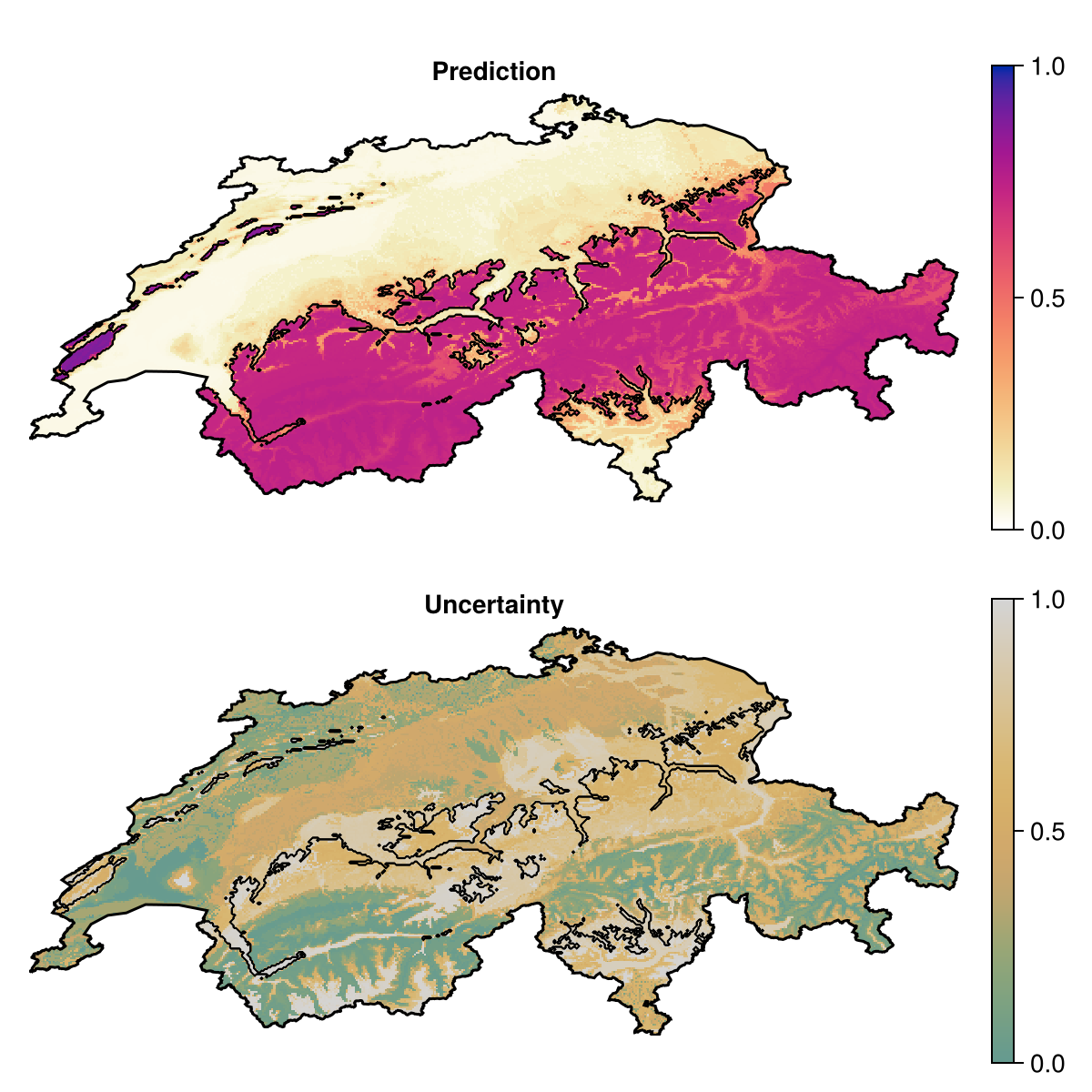

Code for the figure

f = Figure(; size = (600, 600))
ax = Axis(f[1, 1]; aspect = DataAspect(), title = "Prediction")
hm = heatmap!(ax, prd; colormap = :linear_worb_100_25_c53_n256, colorrange = (0, 1))
Colorbar(f[1, 2], hm)
contour!(
    ax,
    predict(ensemble, L; consensus = majority);
    color = :black,
    linewidth = 0.5,
)
lines!(ax, CHE; color = :black)
hidedecorations!(ax)
hidespines!(ax)
ax2 = Axis(f[2, 1]; aspect = DataAspect(), title = "Uncertainty")
hm =
    heatmap!(ax2, quantize(unc); colormap = :linear_gow_60_85_c27_n256, colorrange = (0, 1))
Colorbar(f[2, 2], hm)
contour!(
    ax2,
    predict(ensemble, L; consensus = majority);
    color = :black,
    linewidth = 0.5,
)
lines!(ax2, CHE; color = :black)
hidedecorations!(ax2)
hidespines!(ax2)

# Heterogeneous ensembles

We can also build ensembles of different models. Let's bring in the model we used in the previous tutorial:

sdm2 = SDM(ZScore, Logistic, L, presencelayer, bgpoints)
variables!(sdm2, [1, 11, 5, 8, 6])
hyperparameters!(classifier(sdm2), :η, 1e-4);
hyperparameters!(classifier(sdm2), :interactions, :all);
hyperparameters!(classifier(sdm2), :epochs, 10_000);

As well as a Naive Bayes classifier:

sdm3 = SDM(RawData, NaiveBayes, L, presencelayer, bgpoints)
variables!(sdm3, ForwardSelection)

RawData → NaiveBayes → P(x) ≥ 0.03

These models can all be merged into an heterogeneous ensemble:

hens = Ensemble(sdm2, sdm3)
train!(hens)

An ensemble model with:
	 ZScore → Logistic → P(x) ≥ 0.318
	 RawData → NaiveBayes → P(x) ≥ 0.03

Heterogeneous ensembles can be used in the exact same way as bagged models, so we can for example predict the range according to the three models:

p_range = predict(hens, L; threshold = true, consensus = majority)

🗺️  A 240 × 546 layer with 70065 Bool cells
   Projection: +proj=longlat +datum=WGS84 +no_defs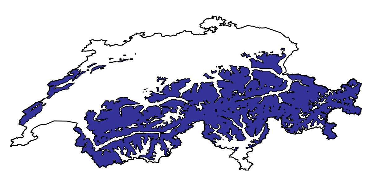

Code for the figure

f = Figure(; size = (600, 300))
ax = Axis(f[1, 1]; aspect = DataAspect())
hm = heatmap!(ax, p_range; colormap = Reverse(:terrain), colorrange = (0, 1))
contour!(ax, p_range; color = :black, linewidth = 0.5)
lines!(ax, CHE; color = :black)
hidedecorations!(ax)
hidespines!(ax)