Using SDeMo with other packages

In this tutorial, we will work on the same species and location as in the excellent tutorial on SDMs by Damaris Zurell, to show how SpeciesDistributionToolkit integrates prediction to the rest of the workflow.

using SpeciesDistributionToolkit
using CairoMakie
using Statistics

Note that there are several sections about the SDeMo package in the "How-to" section of the manual.

Getting the data

CHE = SpeciesDistributionToolkit.openstreetmap("Switzerland");

In order to simplify the code, we will start from a list of bioclim variables that have been picked to optimize the model - SDeMo offers many functions for variable selection.

bio_vars = [1, 11, 5, 8, 6]

5-element Vector{Int64}:
  1
 11
  5
  8
  6

We get the data on these variables from CHELSA2:

provider = RasterData(CHELSA2, BioClim)
L = SDMLayer{Float32}[
    SDMLayer(
        provider;
        layer = x,
        SpeciesDistributionToolkit.boundingbox(CHE)...,
    ) for x in bio_vars
];

And we then clip and trim to the polygon describing Switzerland:

mask!(L, CHE)

5-element Vector{SDMLayer{Float32}}:
 🗺️  A 240 × 546 layer (70065 Float32 cells)
 🗺️  A 240 × 546 layer (70065 Float32 cells)
 🗺️  A 240 × 546 layer (70065 Float32 cells)
 🗺️  A 240 × 546 layer (70065 Float32 cells)
 🗺️  A 240 × 546 layer (70065 Float32 cells)

The next step is to get the data, using the eBird dataset:

ouzel = taxon("Turdus torquatus")
presences = occurrences(
    ouzel,
    first(L),
    "occurrenceStatus" => "PRESENT",
    "limit" => 300,
    "datasetKey" => "4fa7b334-ce0d-4e88-aaae-2e0c138d049e",
)
while length(presences) < count(presences)
    occurrences!(presences)
end

And after this, we prepare a layer with presence data:

presencelayer = mask(first(L), Occurrences(mask(presences, CHE)))

🗺️  A 240 × 546 layer with 70065 Bool cells
   Projection: +proj=longlat +datum=WGS84 +no_defs

The next step is to generate a pseudo-absence mask. We will sample based on the distance to an observation, by also preventing pseudo-absences to be less than 4km from an observation:

background = pseudoabsencemask(DistanceToEvent, presencelayer)
bgpoints = backgroundpoints(nodata(background, d -> d < 4), 2sum(presencelayer))

🗺️  A 240 × 546 layer with 45362 Bool cells
   Projection: +proj=longlat +datum=WGS84 +no_defs

We can take a minute to visualize the dataset, as well as the location of presences and pseudo-absences:

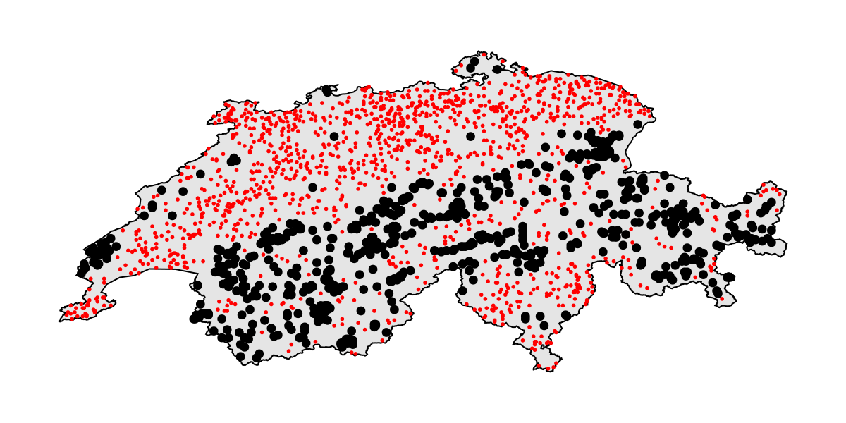
Code for the figure

f = Figure(; size = (600, 300))
ax = Axis(f[1, 1]; aspect = DataAspect())
poly!(ax, CHE; color = :grey90, strokecolor = :black, strokewidth = 1)
scatter!(ax, presencelayer; color = :black)
scatter!(ax, bgpoints; color = :red, markersize = 4)
hidedecorations!(ax)
hidespines!(ax)

Setting up the model

These steps are documented as part of the SDeMo documentation. The only difference here is that rather than passing a matrix of features and a vector of labels, we give a vector of layers (features), and the two layers for presences and absences:

sdm = SDM(ZScore, Logistic, L, presencelayer, bgpoints)
hyperparameters!(classifier(sdm), :η, 1e-4);
hyperparameters!(classifier(sdm), :interactions, :all);
hyperparameters!(classifier(sdm), :epochs, 10_000);

We will now train the model on all the training data.

train!(sdm)

ZScore → Logistic → P(x) ≥ 0.318

Making the first prediction

We can predict using the model by giving a vector of layers as an input. This will return the output as a layer as well:

prd = predict(sdm, L; threshold = false)

🗺️  A 240 × 546 layer with 70065 Float64 cells
   Projection: +proj=longlat +datum=WGS84 +no_defs

Because this prediction is a layer, we can plot it directly:

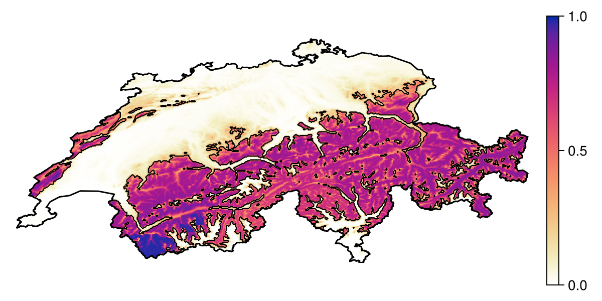
Code for the figure

f = Figure(; size = (600, 300))
ax = Axis(f[1, 1]; aspect = DataAspect())
hm = heatmap!(ax, prd; colormap = :linear_worb_100_25_c53_n256, colorrange = (0, 1))
contour!(ax, predict(sdm, L); color = :black, linewidth = 0.5)
Colorbar(f[1, 2], hm)
lines!(ax, CHE; color = :black)
hidedecorations!(ax)
hidespines!(ax)

As a rule, most relevant function in SDeMo will, when given layers as an argument, return the output as layers:

partial1 = partialresponse(sdm, L, 1; threshold=false)

🗺️  A 240 × 546 layer with 70065 Float64 cells
   Projection: +proj=longlat +datum=WGS84 +no_defs

The output can be visualised as well. Partial responses are given in the same units as the prediction.

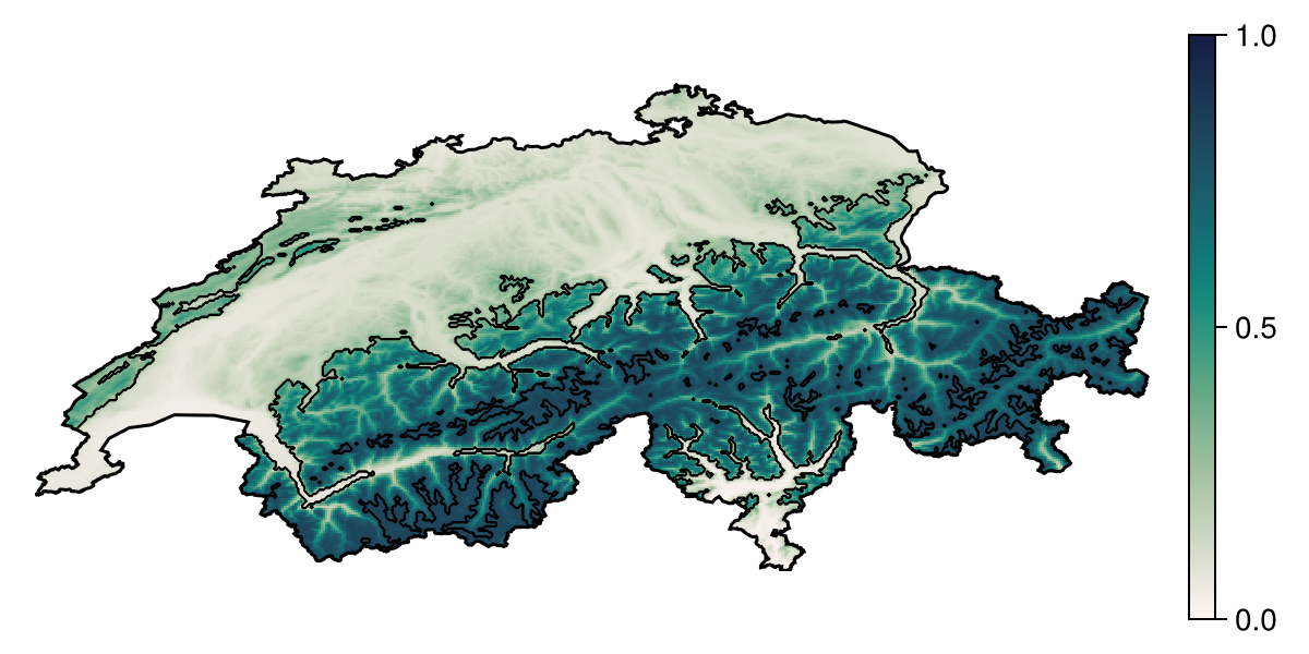
Code for the figure

f = Figure(; size = (600, 300))
ax = Axis(f[1, 1]; aspect = DataAspect())
hm = heatmap!(ax, partial1; colormap = :tempo, colorrange = (0, 1))
contour!(ax, predict(sdm, L); color = :black, linewidth = 0.5)
Colorbar(f[1, 2], hm)
lines!(ax, CHE; color = :black)
hidedecorations!(ax)
hidespines!(ax)

This, naturally, is also true for Shapley values:

shapley1 = explain(sdm, L, 1; threshold=false)

🗺️  A 240 × 546 layer with 70065 Float64 cells
   Projection: +proj=longlat +datum=WGS84 +no_defs

Note that the Shapley values are expressed as a deviation from the average prediction, and so positive values correspond to the presence class being more likely.

Both the explain and partialresponse functions can accept keywords that are passed to predict - in this tutorial, we use threshold=false to provide an explanation on the score returned by the model, but we can also request an explanation of the binary response (this is usually less informative).

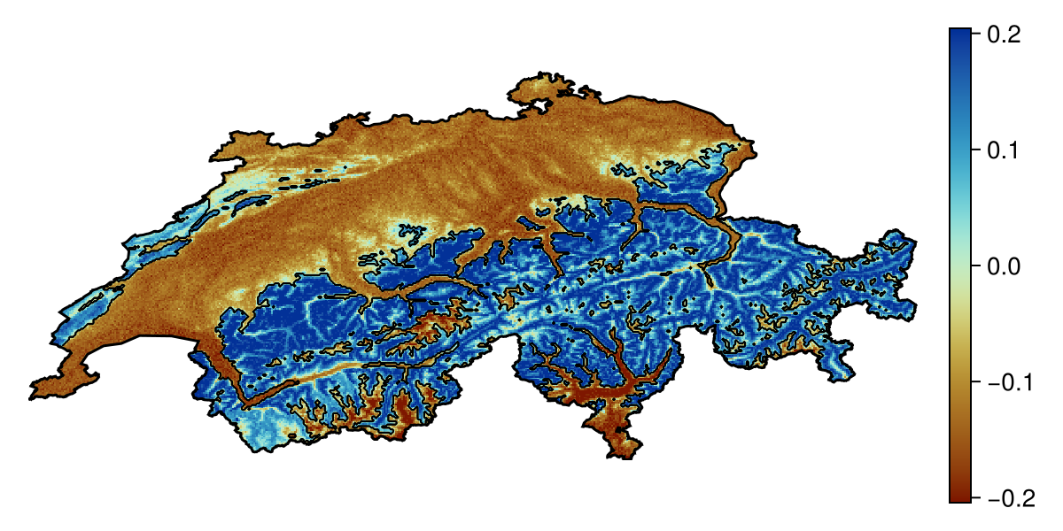
Code for the figure

col_lims = maximum(abs.(quantile(shapley1, [0.1, 0.9]))).*(-1, 1)
f = Figure(; size = (600, 300))
ax = Axis(f[1, 1]; aspect = DataAspect())
hm = heatmap!(ax, shapley1; colormap = :roma, colorrange = col_lims)
contour!(ax, predict(sdm, L); color = :black, linewidth = 0.5)
Colorbar(f[1, 2], hm)
lines!(ax, CHE; color = :black)
hidedecorations!(ax)
hidespines!(ax)

When given a vector of layers, the explain function will return a layer with the explanation for each input variable:

S = explain(sdm, L; threshold=false)

5-element Vector{SDMLayer{Float64}}:
 🗺️  A 240 × 546 layer (70065 Float64 cells)
 🗺️  A 240 × 546 layer (70065 Float64 cells)
 🗺️  A 240 × 546 layer (70065 Float64 cells)
 🗺️  A 240 × 546 layer (70065 Float64 cells)
 🗺️  A 240 × 546 layer (70065 Float64 cells)

We can then put this object into the mosaic function to get the index of which variable is the most important for each pixel:

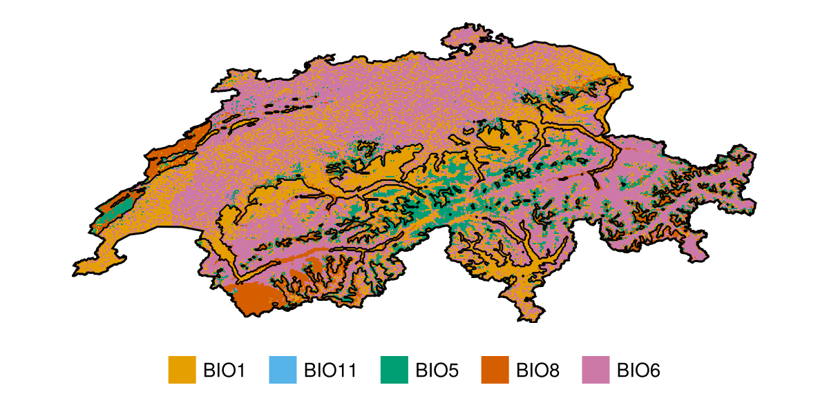
Code for the figure

f = Figure(; size = (600, 300))
mostimp = mosaic(argmax, map(x -> abs.(x), S))
colmap = [colorant"#E69F00", colorant"#56B4E9", colorant"#009E73", colorant"#D55E00", colorant"#CC79A7"]
ax = Axis(f[1, 1]; aspect = DataAspect())
heatmap!(ax, mostimp; colormap = colmap)
contour!(
    ax,
    predict(sdm, L);
    color = :black,
    linewidth = 0.5,
)
lines!(ax, CHE; color = :black)
hidedecorations!(ax)
hidespines!(ax)
Legend(
    f[2, 1],
    [PolyElement(; color = colmap[i]) for i in 1:length(bio_vars)],
    ["BIO$(b)" for b in bio_vars];
    orientation = :horizontal,
    nbanks = 1,
    framevisible = false,
    vertical = false,
)