Generating virtual species

In this vignette, we provide a demonstration of how the different SpeciesDistributionToolkit functions can be chained together to rapidly create a virtual species, generate its range map, and sample points from it according to the predicted suitability.

Note that the generation of virtual species is its own domain of research (Meynard and Kaplan, 2013), and this tutorial is only meant to show how the functions in the package can be made to work together.

julia

using SpeciesDistributionToolkit
using CairoMakie
using Statistics

We start by defining the extent in which we want to create the virtual species. For the purpose of this example, we will use the country of Paraguay. Note that the boundingbox function returns the coordinates in WGS84.

julia

place = getpolygon(PolygonData(OpenStreetMap, Places); place = "Paraguay")
extent = SpeciesDistributionToolkit.boundingbox(place)

(left = -62.64066696166992, right = -54.257999420166016, bottom = -27.606393814086914, top = -19.287647247314453)

We then download some environmental data. In this example, we use the BioClim variables as distributed by CHELSA. In order to simplify the code, we will only use BIO1 (mean annual temperature) and BIO12 (total annual precipitation). Note that we collect these layers in a vector typed as SDMLayer{Float32}, in order to ensure that future operations already receive floating point values.

julia

provider = RasterData(CHELSA2, BioClim)
L = SDMLayer{Float32}[SDMLayer(provider; layer = l, extent...) for l in ["BIO1", "BIO12"]]

2-element Vector{SDMLayer{Float32}}:
 🗺️  A 999 × 1007 layer (1005993 Float32 cells)
 🗺️  A 999 × 1007 layer (1005993 Float32 cells)

We now mask the layers using the polygons we downloaded initially. At the same time, we will transform their values so that they are all in the unit range.

julia

rescale!.(mask!(L, place))

2-element Vector{SDMLayer{Float32}}:
 🗺️  A 999 × 1007 layer (508483 Float32 cells)
 🗺️  A 999 × 1007 layer (508483 Float32 cells)

In the next steps, we will generate some virtual species. These are defined by an environmental response to each layer, linking the value of the layer at a point to the suitability score. For the sake of expediency, we only use logistic responses, and generate one function for each layer (drawing α from a normal distribution, and β uniformly).

julia

logistic(x, α, β) = 1 / (1 + exp((x - β) / α))
logistic(α, β) = (x) -> logistic(x, α, β)

logistic (generic function with 2 methods)

We will next write a function that will sample a value in each layer to serve as the center of the logistic response, draw a shape parameter at random, and then return the suitability of the environment for a virtual species under the assumption of a set prevalence:

julia

function virtualspecies(L::Vector{<:SDMLayer}; prevalence::Float64 = 0.25)
    prevalence = clamp(prevalence, eps(), 1.0)
    invalid = true
    while invalid
        centers = [rand(values(l)) for l in L]
        shapes = randn(length(L))
        predictors = [logistic(centers[i], shapes[i]) for i in eachindex(L)]
        predictions = [predictors[i].(L[i]) for i in eachindex(L)]
        rescale!.(predictions)
        global prediction = prod(predictions)
        #rescale!(prediction)
        invalid = any(isnan, prediction)
    end
    cutoff = quantile(prediction, 1 - prevalence)
    return prediction, cutoff, prediction .>= cutoff
end

virtualspecies (generic function with 1 method)

We can now apply this new function to create a simulated species distribution:

julia

vsp, τ, vrng = virtualspecies(L; prevalence = 0.33)

(🗺️  A 999 × 1007 layer (508483 Float64 cells), 0.04390402910717462, 🗺️  A 999 × 1007 layer (508483 Bool cells))

We can plot the output of this function to inspect what the generated range looks like:

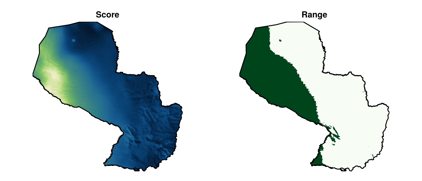
Code for the figure

julia

f = Figure(; size = (700, 300))
ax1 = Axis(f[1, 1]; aspect = DataAspect(), title = "Score")
ax2 = Axis(f[1, 2]; aspect = DataAspect(), title = "Range")
heatmap!(ax1, vsp; colormap = :navia)
heatmap!(ax2, vrng; colormap = :Greens)
for ax in [ax1, ax2]
    tightlimits!(ax)
    hidedecorations!(ax)
    hidespines!(ax)
    lines!(ax, place; color = :black)
end

Random observations for the virtual species are generated by setting the probability of inclusion to 0 for all values above the cutoff, and then sampling proportionally to the suitability for all remaining points. Note that the method is called backgroundpoints, as it is normally used for pseudo-absences. The second argument of this method is the number of points to generate.

julia

presencelayer = backgroundpoints(mask(vsp, nodata(vrng, false)), 100)

🗺️  A 999 × 1007 layer with 167800 Bool cells
   Projection: +proj=longlat +datum=WGS84 +no_defs

We can finally plot the result:

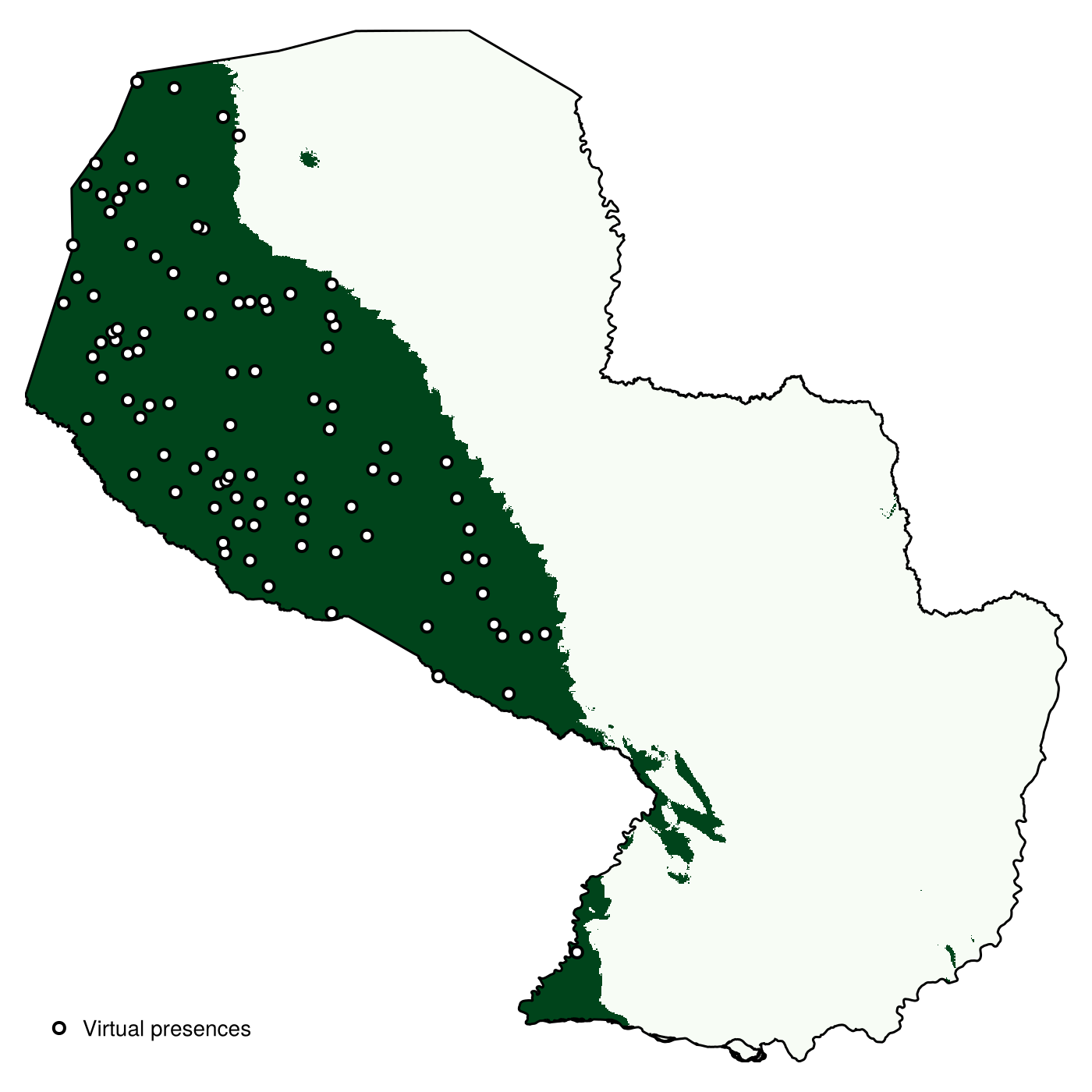
Code for the figure

julia

f = Figure(; size = (700, 700))
ax = Axis(f[1, 1]; aspect = DataAspect())
heatmap!(ax, vrng; colormap = :Greens)
lines!(ax, place; color = :black)
scatter!(
    ax,
    presencelayer;
    color = :white,
    strokecolor = :black,
    strokewidth = 2,
    markersize = 10,
    label = "Virtual presences",
)
tightlimits!(ax)
hidespines!(ax)
hidedecorations!(ax)
axislegend(ax; position = :lb, framevisible = false)

These data could, for example, be used to benchmark species distribution models. Here, in order to say something about potential patterns of biodiversity, we will simulate 100 species, with prevalences drawn uniformly in the unit interval.

julia

ranges = [virtualspecies(L; prevalence = rand())[3] for _ in 1:100]
first(ranges)

🗺️  A 999 × 1007 layer with 508483 Bool cells
   Projection: +proj=longlat +datum=WGS84 +no_defs

We can sum these layers to obtain a measurement of the simulated species richness:

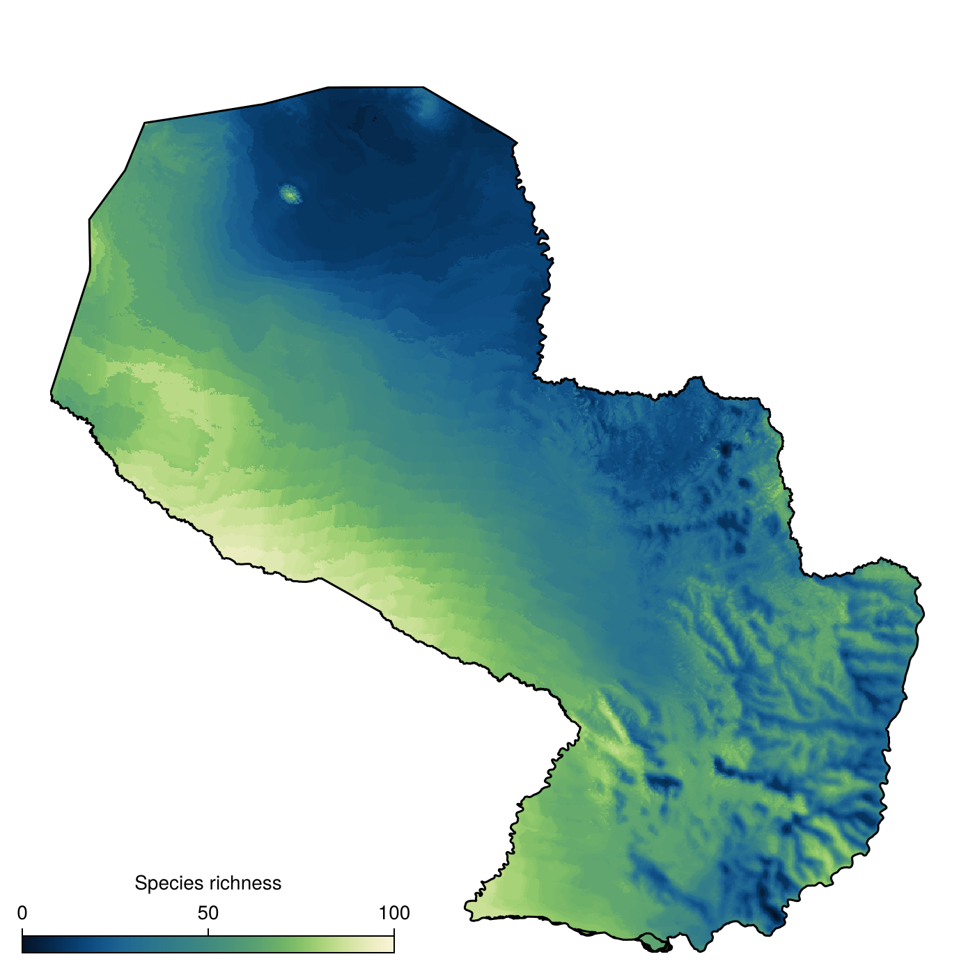
Code for the figure

julia

f = Figure(; size = (700, 700))
richness = mosaic(sum, ranges)
ax = Axis(f[1, 1]; aspect = DataAspect())
hm = heatmap!(ax, richness; colorrange = (0, length(ranges)), colormap = :navia)
Colorbar(
    f[1, 1],
    hm;
    label = "Species richness",
    alignmode = Inside(),
    width = Relative(0.4),
    valign = :bottom,
    halign = :left,
    tellheight = false,
    tellwidth = false,
    vertical = false,
)
hidedecorations!(ax)
lines!(ax, place; color = :black)
hidespines!(ax)

We can now transform these data into a partition of the contribution of each species and location to the total beta-diversity (Legendre and De Cáceres, 2013):

julia

function LCBD(ranges::Vector{SDMLayer{Bool}}; transformation::Function = identity)
    Y = transformation(hcat(values.(ranges)...))
    S = (Y .- mean(Y; dims = 1)) .^ 2.0
    SStotal = sum(S)
    BDtotal = SStotal / (size(Y, 1) - 1)
    SSj = sum(S; dims = 1)
    SCBDj = SSj ./ SStotal
    SSi = sum(S; dims = 2)
    LCBDi = SSi ./ SStotal
    betadiv = similar(first(ranges), Float32)
    betadiv.grid[findall(betadiv.indices)] .= vec(LCBDi)
    return betadiv, vec(SCBDj), BDtotal
end

LCBD (generic function with 1 method)

For good measure, we will also add a function to perform the Hellinger transformation:

julia

function hellinger(Y::AbstractMatrix{T}) where {T <: Number}
    yi = sum(Y; dims = 2) .+ 1
    return sqrt.(Y ./ yi)
end

hellinger (generic function with 1 method)

We can now apply this function to our simulated ranges. The first output is a layer with the local contributions to beta diversity (LCBD), the second is a vector with the contribution of species, and the last element is the total beta diversity.

julia

βl, βs, βt = LCBD(ranges; transformation = hellinger)

(🗺️  A 999 × 1007 layer (508483 Float32 cells), [0.011765526139563963, 0.026842756420192484, 0.012211850943168465, 0.0022973187958042376, 0.0011018562297433292, 0.010689757118200333, 0.010313793456761174, 0.0032287498480885863, 0.011499837865380162, 0.00833603352174186, 0.020906805494785262, 0.014555548573161792, 0.009550090522714272, 0.008233559418893057, 0.011436932724780923, 0.00891940693630012, 0.0043838645100910244, 0.0006889880488489053, 0.014720183422466032, 0.008759694044861148, 0.01045273627179423, 0.0032339464910429066, 0.012855639243297285, 0.004069619480299629, 0.02496919262234288, 0.0072541208374752525, 0.011486468975501237, 0.003670409734778589, 0.004800298766877761, 0.009482367591992363, 0.013074528125891357, 0.010265578375060955, 0.008145207341236244, 0.005909663913640062, 0.011138478948093153, 0.011560049562741483, 0.0065751962335590395, 0.026724333831493707, 0.0039029780545962586, 0.011041911491321462, 0.015567716972960364, 0.008460613283847418, 0.015945752587718152, 0.009424887692615569, 0.0012090244763974867, 0.011345970726481143, 0.013630089663844503, 0.008409359630606272, 0.01085312961724366, 0.001026884387908743, 0.010719279463718819, 0.011123493601932093, 0.0022333596042957977, 0.009612032118580888, 0.011920795835575735, 0.007305673828106455, 0.010318713950680855, 0.011313507440150004, 0.009507676757456292, 0.012032130689058097, 0.007564777178394499, 0.005966619146673527, 0.0023501120799297405, 0.014259842889336296, 0.013850236531382981, 0.020533861329303515, 0.0106432352815318, 0.010967135637866691, 0.0015993369171748175, 0.007914483886615161, 0.009438342507476556, 0.010236628945323756, 0.014873618545677288, 0.013309760609278716, 0.01160037307142353, 0.00930039339089494, 0.02577060351013607, 0.010763402598156734, 0.009999830123275086, 0.021669483409308212, 0.0026631077900581015, 0.010870075106619257, 0.0049759484888276685, 0.012184590642677968, 0.011108810090272139, 0.007799845598852312, 0.01603235344894764, 0.009048949489331189, 0.010343465453425396, 0.005512507913422314, 0.013271782319392555, 0.01085442202874547, 0.004558915893028969, 0.011341196497628258, 0.0009913192012942656, 0.011488157454824689, 0.01035787487511841, 0.01057690405977546, 0.0005089862536992864, 0.009883337547137402], 0.36796185798842773)

We can now plot the various elements (most of the code below is actually laying out the sub-panels for the plot), to identify areas in space that contribute most to ecological uniqueness (Dansereau et al., 2022):

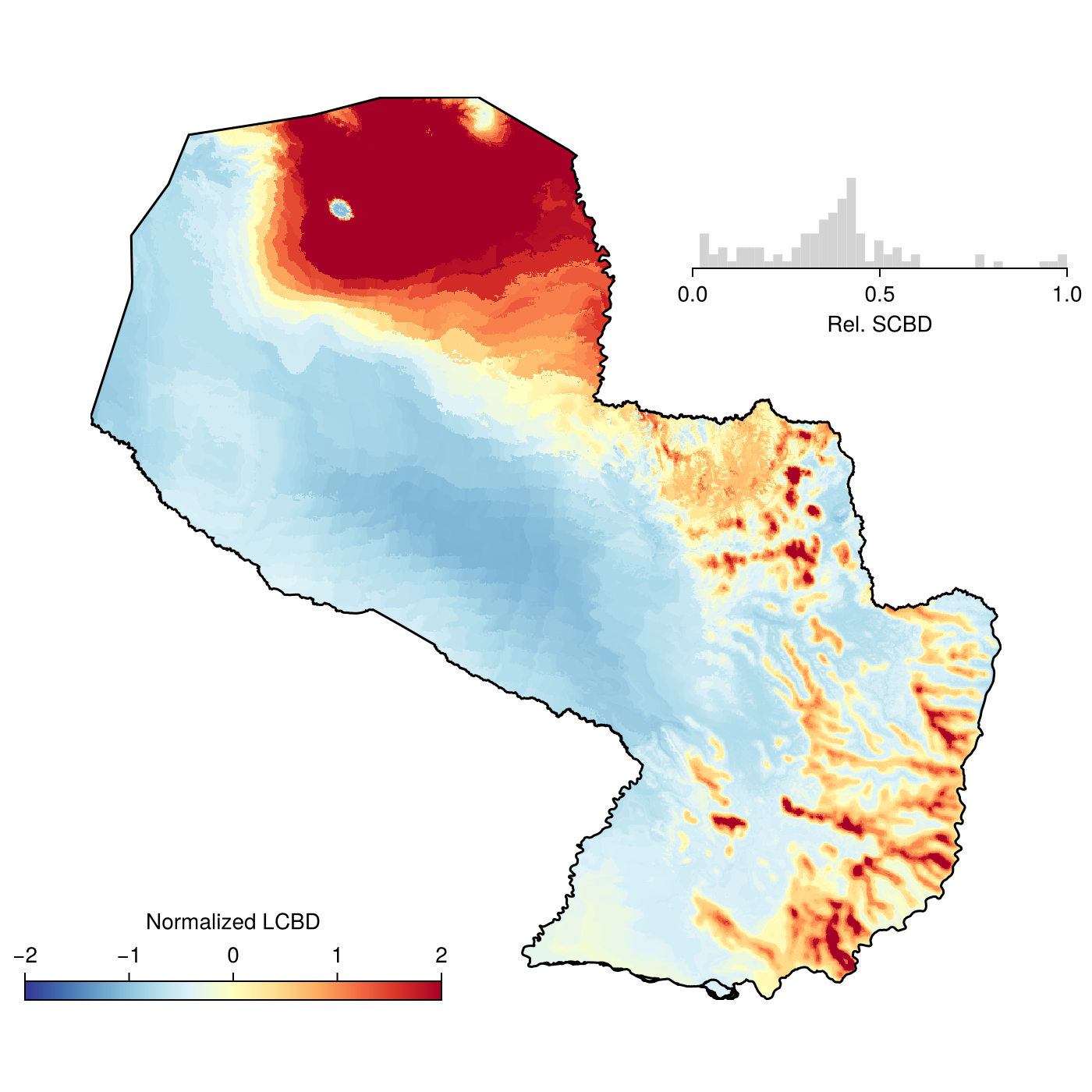
Code for the figure

julia

f = Figure(; size = (700, 700))
ax = Axis(f[1, 1]; aspect = DataAspect())
hm = heatmap!(
    ax,
    (βl - mean(βl)) / std(βl);
    colormap = Reverse(:RdYlBu),
    colorrange = (-2, 2),
)
lines!(ax, place; color = :black)
Colorbar(
    f[1, 1],
    hm;
    label = "Normalized LCBD",
    alignmode = Inside(),
    width = Relative(0.4),
    valign = :bottom,
    halign = :left,
    tellheight = false,
    tellwidth = false,
    vertical = false,
)
tightlimits!(ax)
hidespines!(ax)
hidedecorations!(ax)
ax_inset = Axis(f[1, 1];
    width = Relative(0.36),
    height = Relative(0.1),
    halign = 1.0,
    valign = 0.9,
    xlabel = "Rel. SCBD")
hist!(ax_inset, βs ./ maximum(βs); color = :lightgrey, bins = 40)
xlims!(ax_inset, 0, 1)
hidespines!(ax_inset, :t, :r, :l)
hideydecorations!(ax_inset)
hidexdecorations!(ax_inset; ticks = false, ticklabels = false, label = false)
tightlimits!(ax_inset)

References

Dansereau, G.; Legendre, P. and Poisot, T. (2022). Evaluating ecological uniqueness over broad spatial extents using species distribution modelling. Oikos (Copenhagen, Denmark) 2022, e09063.
Legendre, P. and De Cáceres, M. (2013). Beta diversity as the variance of community data: dissimilarity coefficients and partitioning. Ecology letters 16, 951–963.
Meynard, C. N. and Kaplan, D. M. (2013). Using virtual species to study species distributions and model performance. Journal of biogeography 40, 1–8.

Generating virtual species ​

References ​

Generating virtual species

References