Calibration of SDM outputs

The purpose of this vignette is to show how to calibrate the results of an SDM.

using SpeciesDistributionToolkit
using CairoMakie

We will work on the demo data:

X, y = SDeMo.__demodata()
sdm = SDM(PCATransform, NaiveBayes, X, y)
variables!(sdm, ForwardSelection)

PCATransform → NaiveBayes → P(x) ≥ 0.302

This model returns the following class scores:

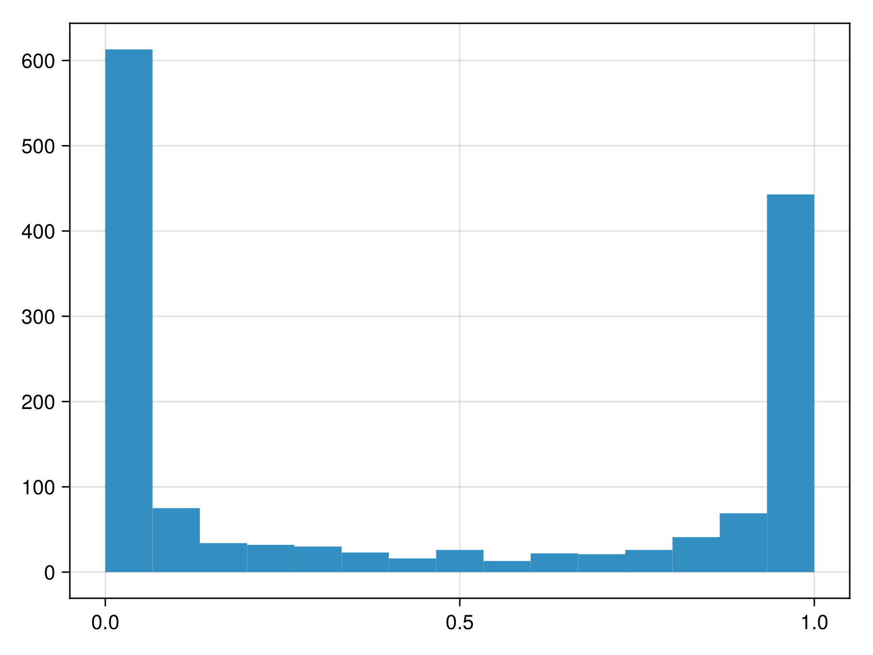
Code for the figure

f = Figure()
ax = Axis(f[1, 1])
hist!(ax, predict(sdm; threshold=false))

To figure out whether these are close to actual probabilities, we can look at the reliability curve

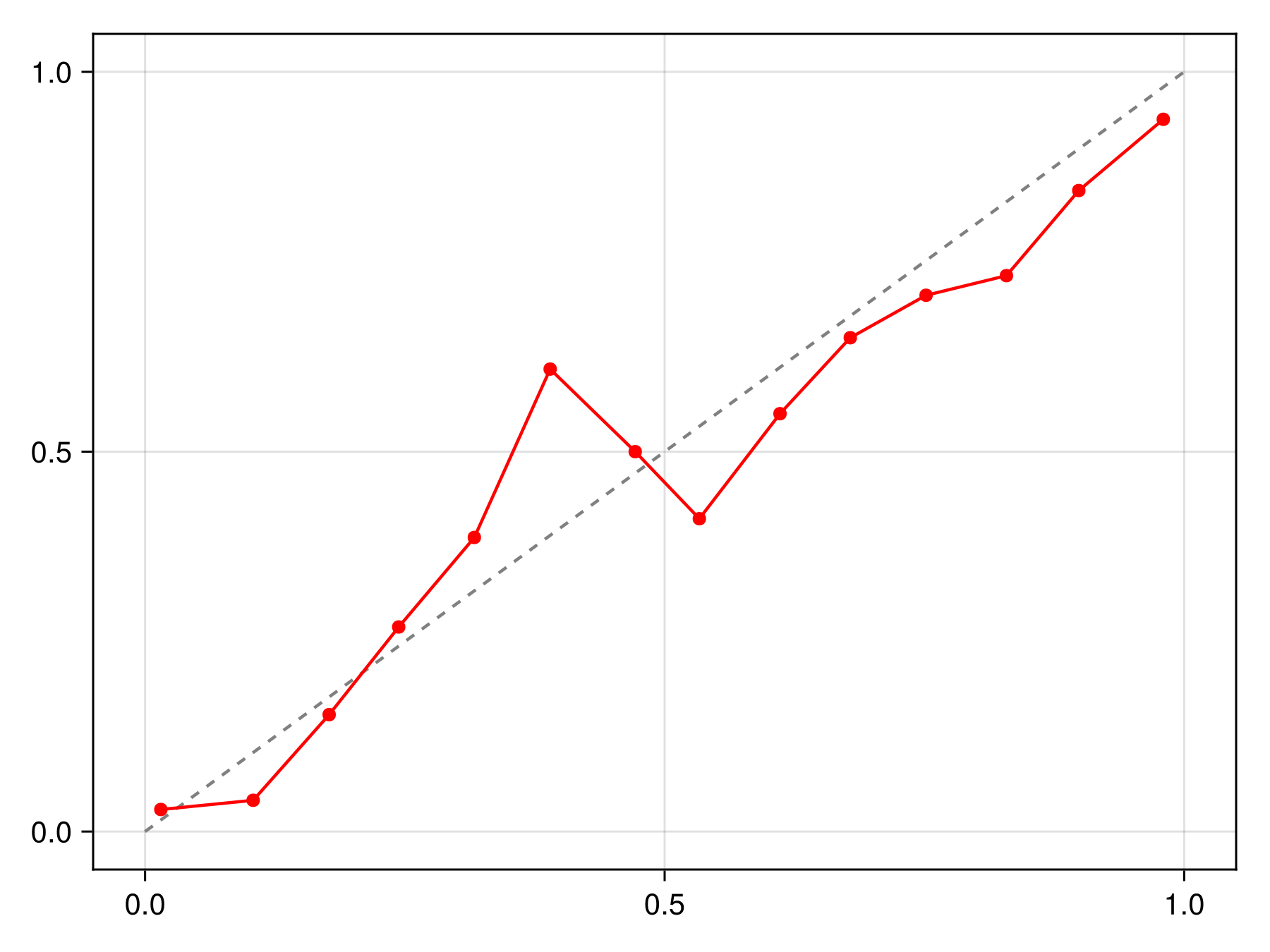
Code for the figure

f = Figure()
ax = Axis(f[1, 1])
lines!(ax, [0, 1], [0, 1], color=:grey, linestyle=:dash)
scatterlines!(ax, reliability(sdm, bins=15)..., color=:red)

We can apply different types of calibration functions, such as for example isotonic regression:

C = calibrate(IsotonicCalibration, sdm)

IsotonicCalibration(SDeMo.var"#evaluate#PAVA##2"{Vector{Float64}, Vector{Float64}}([0.025179856115107913, 0.048, 0.13333333333333333, 0.16216216216216214, 0.3076923076923077, 0.40625, 0.5000000000000001, 0.5714285714285714, 0.6785714285714286, 0.7380952380952381, 0.7777777777777778, 0.868421052631579, 0.8977272727272727, 0.9414893617021277], [0.010446841702334862, 0.059153266991951135, 0.14602746759462176, 0.19011707586999216, 0.2708963211682988, 0.3110931019922129, 0.38464467093945615, 0.5604360184813539, 0.6927670780514079, 0.7706322760279891, 0.8548092612242976, 0.8965091421785246, 0.9418574850997998, 0.9863507703735425, 0.9863507703735425]))

The calibration can be applied by passing it to the correct function, which returns a function to correct a point prediction:

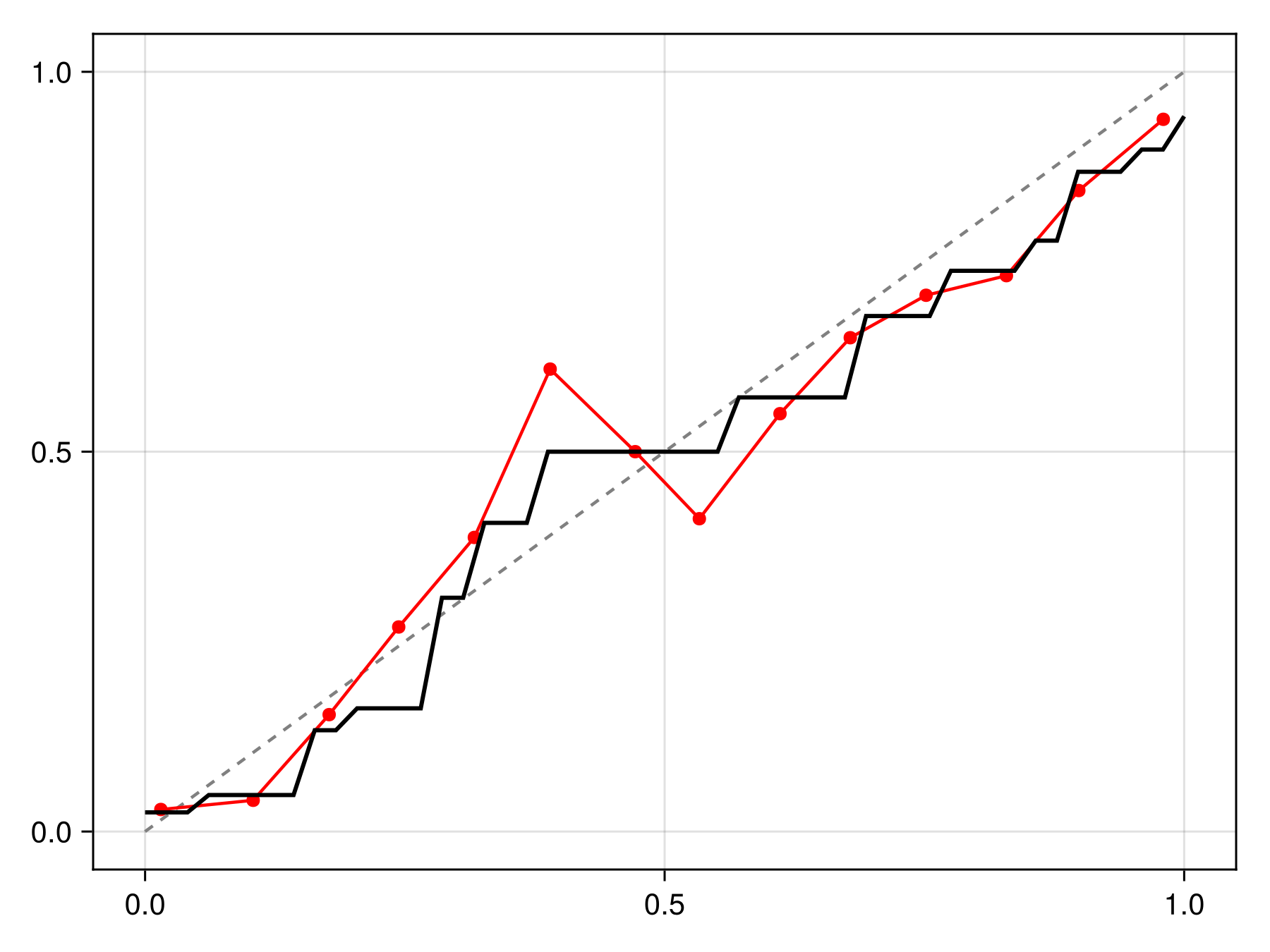
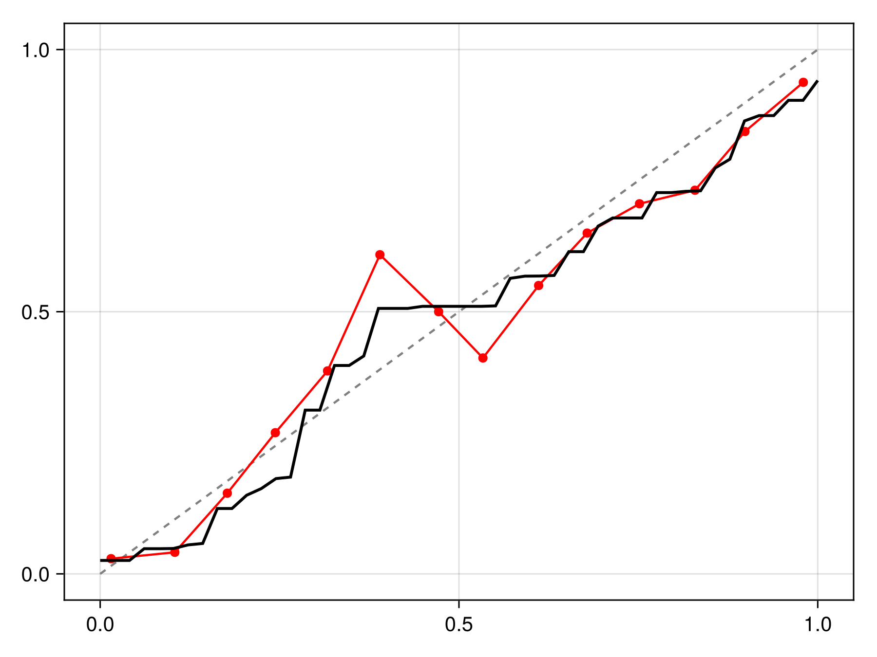
Code for the figure

f = Figure()
x = LinRange(0.0, 1.0, 50)
ax = Axis(f[1, 1])
lines!(ax, [0, 1], [0, 1], color=:grey, linestyle=:dash)
scatterlines!(ax, reliability(sdm, bins=15)..., color=:red)
lines!(ax, x, correct(C).(x), color=:black, linewidth=2)

We can check that this calibration is indeed making the model more reliable compared to the initial version:

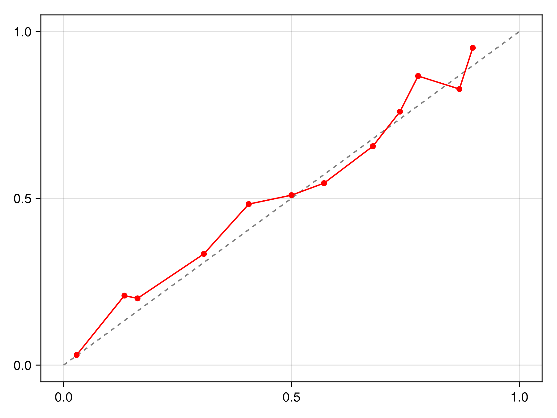
Code for the figure

f = Figure()
x = LinRange(0.0, 1.0, 50)
ax = Axis(f[1, 1])
lines!(ax, [0, 1], [0, 1], color=:grey, linestyle=:dash)
scatterlines!(ax, reliability(sdm, bins=15, link=correct(C))..., color=:red)

It is possible to pass a sample keyword to calibrate to only use a series of training points for calibration. This allows to use multiple samples to estimate the calibration function:

samples = first.(bootstrap(sdm))
C = [calibrate(IsotonicCalibration, sdm; samples=s) for s in samples]
cfunc = correct(C)

#correct##2 (generic function with 1 method)

The correction function will then average the results for each calibration to return the final probability:

Code for the figure

f = Figure()
x = LinRange(0.0, 1.0, 50)
ax = Axis(f[1, 1])
lines!(ax, [0, 1], [0, 1], color=:grey, linestyle=:dash)
scatterlines!(ax, reliability(sdm, bins=15)..., color=:red)
lines!(ax, x, cfunc.(x), color=:black, linewidth=2)

The package also implements Platt's calibration with a fast algorithm, which is appropriate when the relationship between scores and probabilities is sigmoid.