Sliding windows

using SpeciesDistributionToolkit
using CairoMakie
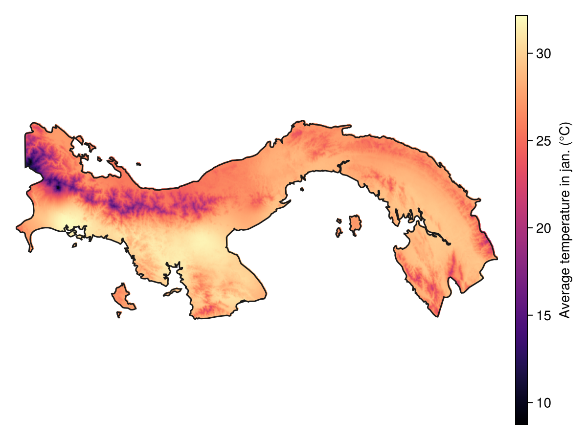
import Statistics

Sliding windows analyses allow to aggregate data within a set distance from a pixel (expressed as a radius, in kilometers) and return this information in a new raster with the same dimension. We will illustrate this by getting the average temperature in january for the country of Uruguay, and identifying places that are coldspots, i.e. colder than their surroundings.

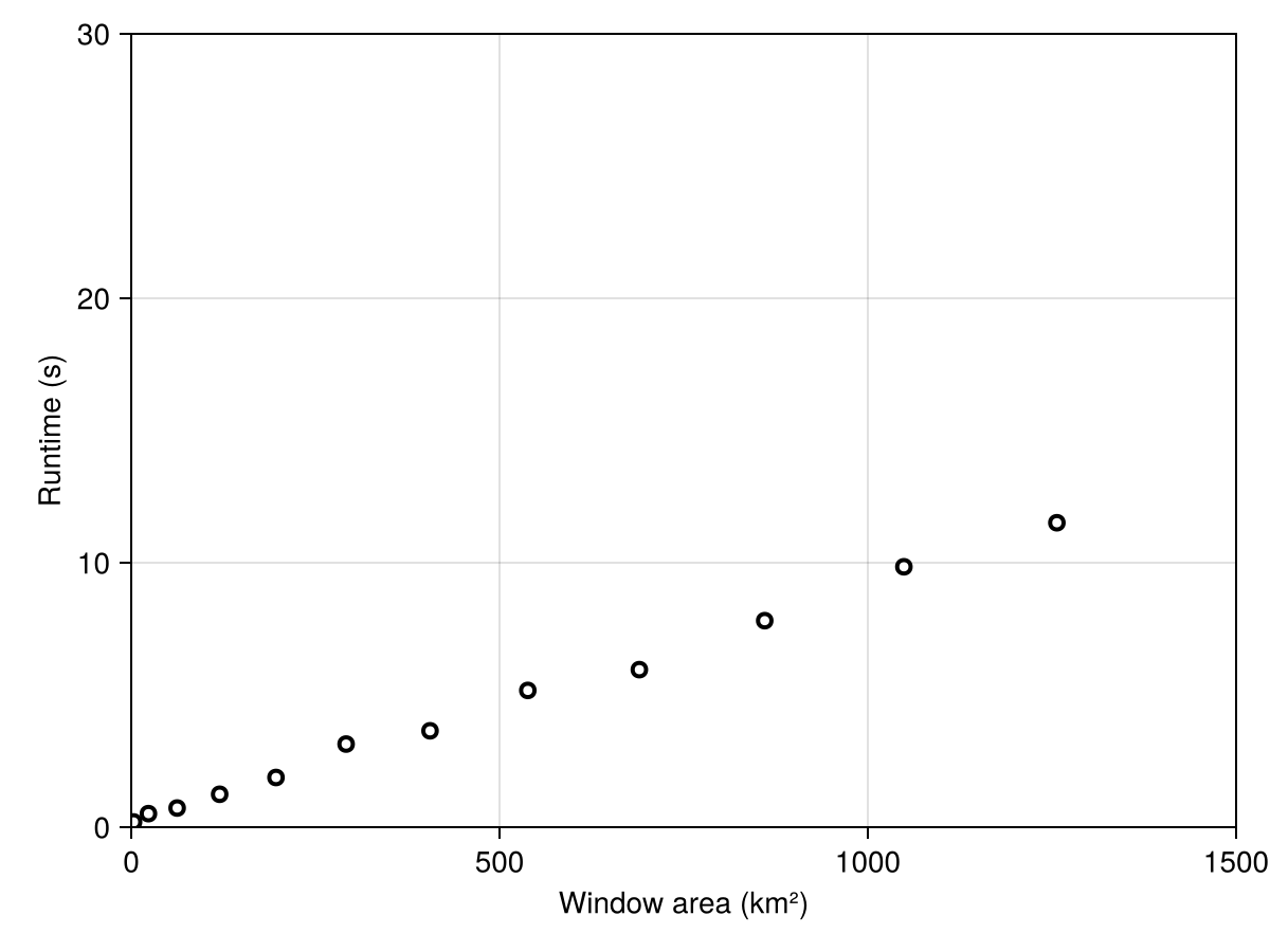
Sliding windows can take time

This analysis requires to identify the pixels around a point that are a set distance from the centerpoint. Internally, the function does some half-smart geometry to figure out the minimum number of operations, but the time required to identify the pixels will scale with the raster resolution and size. The calculation will always use available threads.

region = getpolygon(PolygonData(NaturalEarth, Countries); resolution = 10)["Panama"]
extent = SpeciesDistributionToolkit.boundingbox(region)
temperature = SDMLayer(RasterData(CHELSA2, AverageTemperature); extent...)
mask!(temperature, region)

🗺️  A 292 × 708 layer with 88149 Float64 cells
   Spatial Reference System: +proj=longlat +datum=WGS84 +no_defs

We can now plot the raw data:

Code for the figure

f = Figure()
ax = Axis(f[1, 1]; aspect = DataAspect())
hm = heatmap!(ax, temperature; colormap = :magma)
lines!(ax, region; color = :grey10)
hidedecorations!(ax)
hidespines!(ax)
Colorbar(f[1, 2], hm; label = "Average temperature in jan. (°C)")

We will start by reporting the average temperature within a 12 km radius from any given point:

avg_12km = slidingwindow(Statistics.mean, temperature; radius = 12.0)

🗺️  A 292 × 708 layer with 88149 Float64 cells
   Spatial Reference System: +proj=longlat +datum=WGS84 +no_defs

The radius is always expressed in kilometers. Once the operation is finished, we can look at the results:

Code for the figure

f = Figure()
ax = Axis(f[1, 1]; aspect = DataAspect())
hm = heatmap!(ax, temperature; colormap = :magma, colorrange = extrema(temperature))
lines!(ax, region; color = :grey10)
hidedecorations!(ax)
hidespines!(ax)
Colorbar(f[1, 2], hm; label = "Average temperature in jan. (°C)")

It is important to note that the speed of the function decreases with the radius of the problem. We can illustrate this with a simple (and not very robust) benchmark:

Code for the figure

R = LinRange(1.0, 20.0, 12)
T = zeros(length(R))
destination = copy(temperature)
for (i,r) in enumerate(R)
    started = time()
    slidingwindow!(destination, Statistics.mean, temperature; radius=r)
    finished = time()
    T[i] = finished-started
end
f = Figure()
ax = Axis(f[1, 1]; xlabel="Window area (km²)", ylabel="Runtime (s)")
scatter!(ax, π.*R.^2.0, T, color=:white, strokecolor=:black, strokewidth=2)
xlims!(ax, 0, 1500)
ylims!(ax, 0, 30)
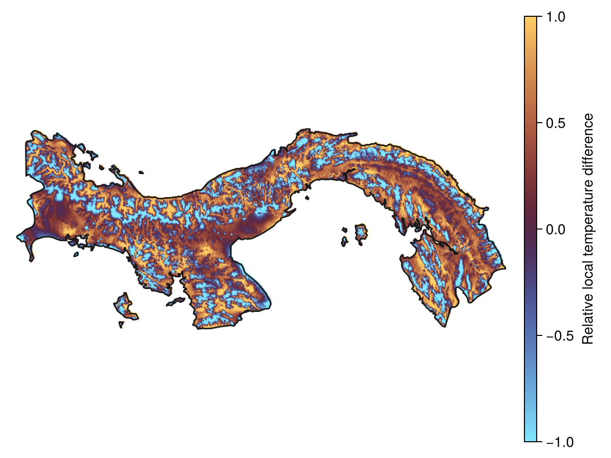
tightlimits!(ax)

To identify coldspots, it would be tempting to repeat this process for the standard deviation, and then combine these three layers into a z-score. But because of the need to identify neighboring pixels, this would be extremely ineffective.

Instead, we will use the centervalue keyword of slidingwindow, which requires that we use a function with two arguments: the value of the reference pixel, and the rest of the values:

zscore(x, v) = (x - Statistics.mean(v)) / Statistics.std(v)

zscore (generic function with 1 method)

We can now get the z-score of temperature around the point in a single call:

z_12km = slidingwindow(zscore, temperature; radius = 12.0, centervalue = true)

🗺️  A 292 × 708 layer with 88149 Float64 cells
   Spatial Reference System: +proj=longlat +datum=WGS84 +no_defs

This layer can be plotted to show which locations are colder/warmer than their surroundings.

Code for the figure

f = Figure()
ax = Axis(f[1, 1]; aspect = DataAspect())
hm = heatmap!(ax, z_12km; colormap = Reverse(:managua), colorrange = (-1, 1))
lines!(ax, region; color = :grey10)
hidedecorations!(ax)
hidespines!(ax)
Colorbar(f[1, 2], hm; label = "Relative local temperature difference")

Related documentation

SimpleSDMLayers.slidingwindow Function

slidingwindow(f::Function, layer::SDMLayer; kwargs...)

Performs a sliding window analysis in which all cells in the returned layer receive the output of applying the function f to all cells in a radius of radius kilometer on the layer layer.

The f function must take a vector of values as an input, and must return a single value as an output. The returned layer will have the type returned by f.

If the centervalue keyword is set to true (default is false), then the f function must take (r, v) an input, where r is the value for the reference cell, and v is the vector of values for all other cells in the window. This is useful to measure, for example, z-scores within a known distance radius: (r,v) -> (r-mean(v))/std(v).

Internally, this function uses threads to speed up calculation quite a bit, and uses the slidingwindow! function.

source

SimpleSDMLayers.slidingwindow! Function

slidingwindow!(destination::SDMLayer, f::Function, layer::SDMLayer; radius::AbstractFloat=100.0)

Performs a sliding window analysis in which all cells in the destination layer receive the output of applying the function f to all cells in a radius of radius kilometer on the layer layer.

The f function must take a vector of value as an input, and must return a single value as an output. The destination layer must have the correct type re. what is returned by f.

If the centervalue keyword is set to true (default is false), then the f function must take (r, v) an input, where r is the value for the reference cell, and v is the vector of values for all other cells in the window. This is useful to measure, for example, z-scores within a known distance radius: (r,v) -> (r-mean(v))/std(v).

Internally, this function uses threads to speed up calculation quite a bit.

source