Operating on polygons

Polygons can be manipulated with various different operations: (1) adding, which returns the union of polygons, (2) subtracting, which returns the difference between two polygons, (3) intersecting, which returns the regions both polygons contain, and (4) inverting, which takes a single polygon and returns a new polygon that encloses all the area within the original polygons bounding box that is not contained in the original polygons.

using SpeciesDistributionToolkit
using CairoMakie

Adding Polygons

Let's start with the simplest version: adding polygons. Let's load the polygons for two US states, Texas and Oklahoma

texas = getpolygon(PolygonData(OpenStreetMap, Places); place = "Texas")
oklahoma = getpolygon(PolygonData(OpenStreetMap, Places); place = "Oklahoma")

FeatureCollection with 1 features, each with 0 properties

We can plot them to show that they are two adjacent states (that don't overlap):

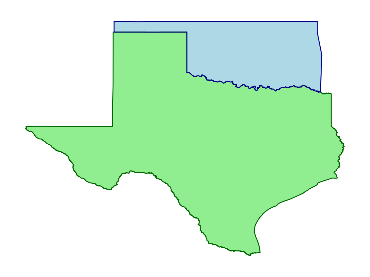
Code for the figure

f, ax, pl = poly(texas; color = :lightgreen)
poly!(oklahoma; color = :lightblue)
lines!(texas; color = :darkgreen)
lines!(oklahoma; color = :darkblue)
hidedecorations!(ax)
hidespines!(ax)

By default, these are both downloaded as FeatureCollections with a single feature. We can add them as FeatureCollections to yield a single polygon that consists of all regions enclosed by both of them.

tex_and_ok = add(texas, oklahoma)

Polygon(Geometry: POLYGON ((-103.00244140625 36.5450782775879,-103.0 ... 246)))

which we can then visualize:

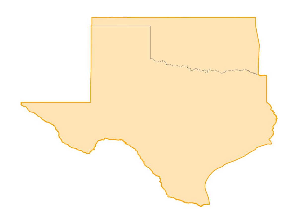
Code for the figure

f, ax, pl = poly(tex_and_ok; color = :moccasin)
lines!(texas; color = :grey50, linewidth = 0.5)
lines!(tex_and_ok; color = :orange)
hidedecorations!(ax)
hidespines!(ax)

We can also do this with the single features directly

add(texas[1], oklahoma[1])

Polygon(Geometry: POLYGON ((-106.635765075684 31.8694763183594,-106. ... 547)))

or the polygons those features contain

add(texas[1].geometry, oklahoma[1].geometry)

Polygon(Geometry: POLYGON ((-106.635765075684 31.8694763183594,-106. ... 547)))

which yields the same result.

Alternatively, we can also just use the + operator, which does that same thing as add:

texas + oklahoma

Polygon(Geometry: POLYGON ((-103.00244140625 36.5450782775879,-103.0 ... 246)))

Sometimes we may have FeatureCollections with more than one feature. For example, lets combine Texas and Oklahoma FeatureCollections with vcat

vcat(texas, oklahoma)

FeatureCollection with 2 features, each with 0 properties

We'll also load another state to combine

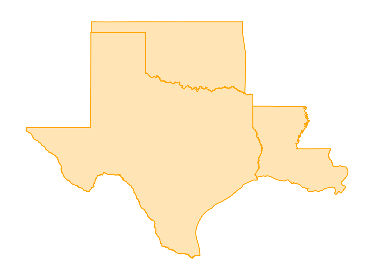
louisiana = getpolygon(PolygonData(OpenStreetMap, Places); place = "Louisiana")

FeatureCollection with 1 features, each with 0 properties

By default, add unions all features within collections too, e.g. the following creates a single polygon with the entire area of all three states

tx_ok_la = texas + oklahoma + louisiana

Polygon(Geometry: POLYGON ((-91.6628646850586 29.3747406005859,-91.6 ... 722)))

We can look at the output (the state lines have been added, and are in light grey):

Code for the figure

f, ax, pl = poly(tx_ok_la; color = :moccasin)
lines!(texas; color = :grey50, linewidth = 0.5)
lines!(oklahoma; color = :grey50, linewidth = 0.5)
lines!(louisiana; color = :grey50, linewidth = 0.5)
lines!(tx_ok_la; color = :orange)
hidedecorations!(ax)
hidespines!(ax)

If we want to keep their separate boundaries, we should use vcat:

tx_ok_la_separate = vcat(texas, oklahoma, louisiana)

FeatureCollection with 3 features, each with 0 properties

And plot to show they keep their individual boundaries

Code for the figure

f, ax, pl = poly(tx_ok_la_separate; color = :moccasin)
lines!(tx_ok_la_separate; color = :orange)
hidedecorations!(ax)
hidespines!(ax)

This covers the addition of polygons.

Subtracting polygons

We subtract polygons in a similar way. The method subtract(x, y) removes the area contained in y from x. For example, let's remove the two largest metropolitan regions from Texas, first by loading them

dallas = getpolygon(PolygonData(OpenStreetMap, Places); place = "Dallas")
houston = getpolygon(PolygonData(OpenStreetMap, Places); place = "Houston")

FeatureCollection with 1 features, each with 0 properties

We can use subtract on them iteratively

rural_texas = texas
rural_texas = subtract(rural_texas, dallas)
rural_texas = subtract(rural_texas, houston)

Polygon(Geometry: POLYGON ((-106.635757446289 31.8721027374268,-106. ... 664)))

and visualize:

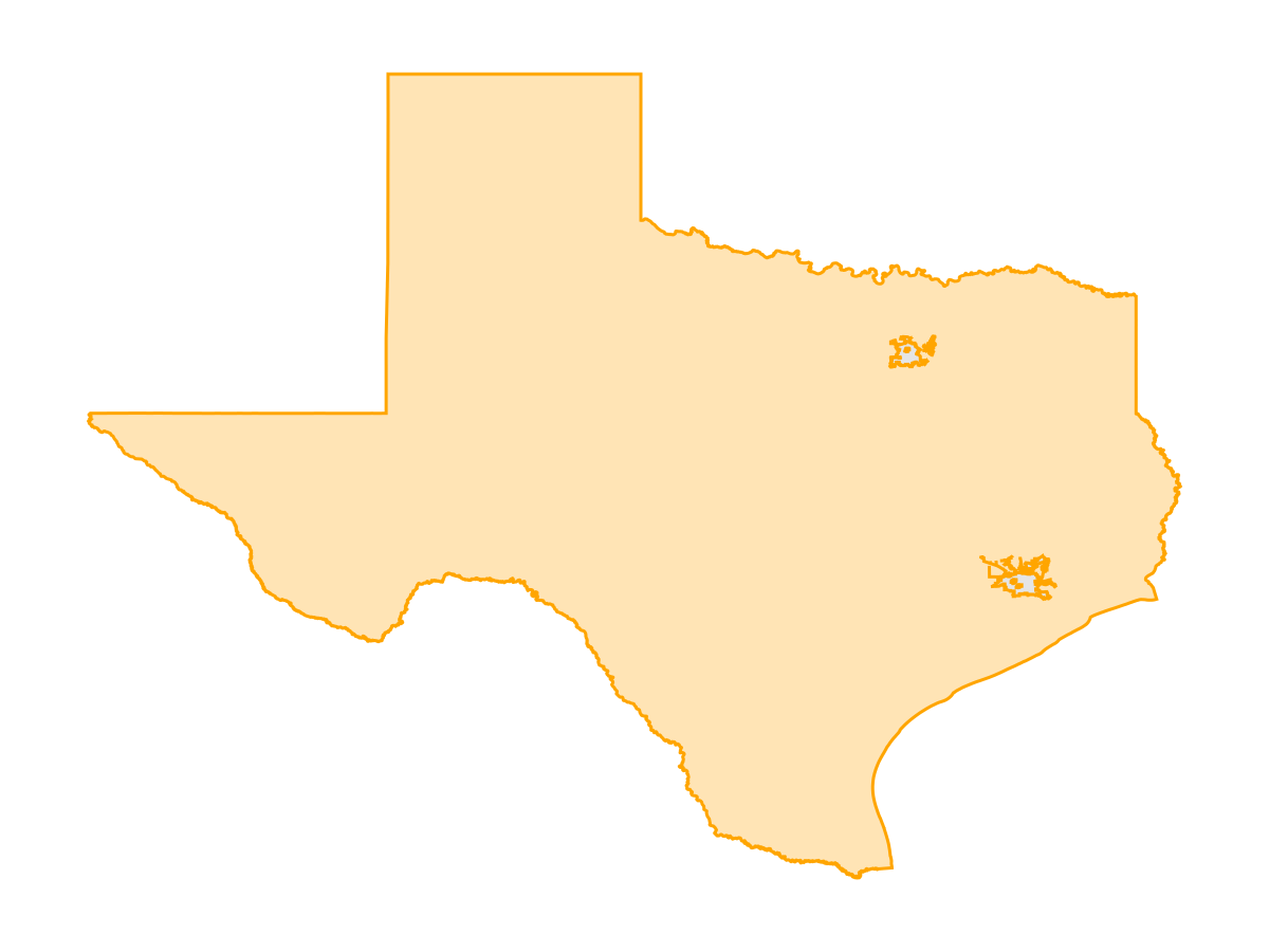
Code for the figure

f, ax, pl = poly(rural_texas; color = :moccasin)
poly!(dallas; color = :grey90)
poly!(houston; color = :grey90)
lines!(rural_texas; color = :orange)
hidedecorations!(ax)
hidespines!(ax)

Or in a single line using the - operator

rural_texas = texas - (dallas + houston)

FeatureCollection with 1 features, each with 0 properties

which results in the same thing:

Code for the figure

f, ax, pl = poly(rural_texas; color = :moccasin)
poly!(dallas + houston; color = :grey90)
lines!(rural_texas; color = :orange)
hidedecorations!(ax)
hidespines!(ax)

These operations can be chained to perform more complex clipping.

Intersecting a Polygon

We can also use the intersect method to extract the region where two polygons intersect.

As an example, let's consider trying to make a map of Texas, which different polygons corresponding to different ecoregions. We'll start by downloading the EPA North America level 3 ecoregions

ecoregions = getpolygon(PolygonData(EPA, Ecoregions); level = 2)

FeatureCollection with 51 features, each with 2 properties

and then intersect them

tx_ecoregions = intersect(texas, ecoregions)

FeatureCollection with 6 features, each with 2 properties

and visualize the different ecoregions in texas

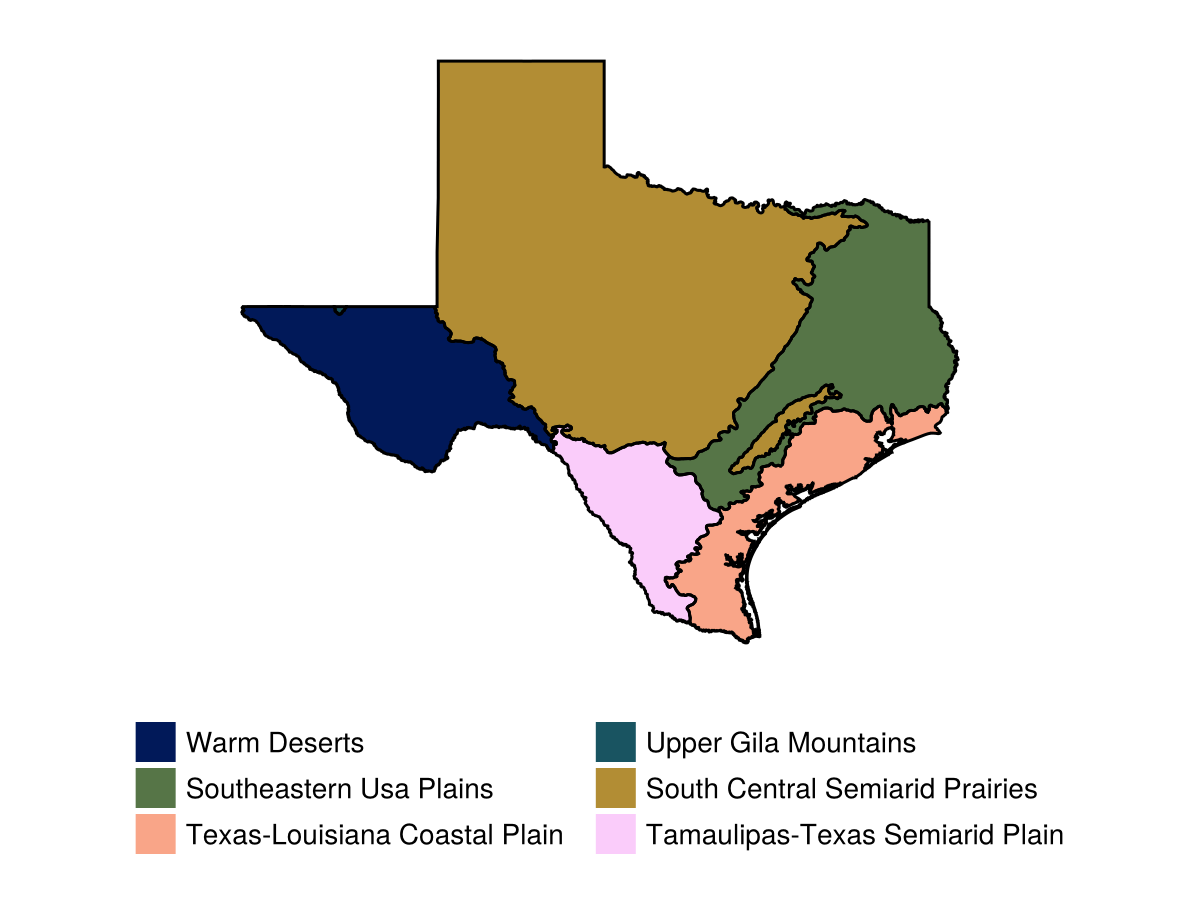
Code for the figure

c = cgrad(:batlow10, length(tx_ecoregions); categorical = true)
f = Figure()
ax = Axis(f[1, 1]; aspect = DataAspect())
for (i, ecoregion) in enumerate(tx_ecoregions)
    poly!(ax, ecoregion; label = titlecase(ecoregion.properties["Name"]), color = c[i])
end
lines!(ax, tx_ecoregions; color = :black)
hidedecorations!(ax)
hidespines!(ax)
Legend(f[2, 1], ax; framevisible = false, nbanks = 2, tellwidth = false, tellheight = false)
rowsize!(f.layout, 2, Relative(0.2))

Finally, we can clip a series of polygons with a boundingbox:

bbox = (left = -100.0, right = -95.0, bottom = 27.5, top = 32.5)

tx_clip = clip(tx_ecoregions, bbox)

FeatureCollection with 4 features, each with 2 properties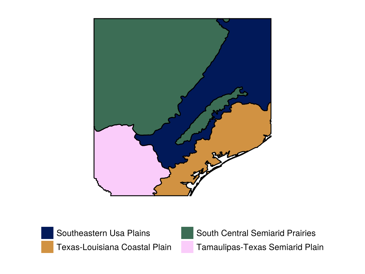

Code for the figure

c = cgrad(:batlow10, length(tx_clip); categorical = true)
f = Figure()
ax = Axis(f[1, 1]; aspect = DataAspect())
for (i, ecoregion) in enumerate(tx_clip)
    poly!(ax, ecoregion; label = titlecase(ecoregion.properties["Name"]), color = c[i])
end
lines!(ax, tx_clip; color = :black)
hidedecorations!(ax)
hidespines!(ax)
Legend(f[2, 1], ax; framevisible = false, nbanks = 2, tellwidth = false, tellheight = false)
rowsize!(f.layout, 2, Relative(0.2))

Chained together, these functions can be used to create the right polygon to clip or mask data.