Background

There is value in being able to identify boundaries within a landscape as it provides us with a starting point from which to understand changes in species assemblages, ecological communities, or even simply to delineate areas (based on a shared property) into discrete units, for example ecosystemic regions (Fortin et al. 2000, Post et al. 2007). Here we present a Julia (Bezanson et al. 2017) package aimed at detecting boundaries across a specified geographical area by identifying zones of rapid change using the wombling edge detection algorithm. This approach was originally developed by Womble (1951) in the context of understanding trait variation within a geographic area and was later modified by Barbujani et al. (1989) for the purpose of understanding changes in gene frequencies, although it also has a more general ecological application with regards to spatial data (Fortin and Dale 2005), serving as a complimentary approach to cluster analysis (Fortin and Drapeau 1995). Wombling has applicability to a wide range scenarios e.g. trait measurements or genotypes (Barbujani et al. 1989), species interaction networks (Fortin et al. 2021), and has explicitly been used (to list a few examples) to detect transitions within a landscape (Camarero et al. 2000, Philibert et al. 2008), and analyse the spread of invasive species (Fitzpatrick et al. 2010). Although the origins of wombling may be rooted in anthropology and has been extensively used in ecology the potential applicability also extends to other systems such as high-energy experiments in physics (Matchev et al. 2020), or to understand the genetic-linguistic patterns of European populations (Sokal et al. 1990).

Broadly speaking spatial wombling is an edge-detection algorithm which traverses a geographic area (for the purpose of this discussion let’s imagine a spatially referenced dataset pertaining to species richness for each location) and defines this area in terms of the rate (m) and corresponding direction of change (θ) through interpolating between nearest neighbours. Although the wombling algorithm (as implemented here) is designed to work with two-dimensional i.e. planar data (as delimited by x and y — which would be the co-ordinates of where species richness was sampled), it is beneficial to view this plane as a three-dimensional object (or series of curves), as shown in fig. 1, panel A. Here the ‘amplitude’ of the curvature of the plane is determined by the value of z (species richness) and the rate and direction of change is calculated by using the first-order partial derivative (∂) of the surface (curve) as described by f(x,y). This then gives us an indication of how steep the gradient/curve (m) is between neighbouring cells as well as the direction (from the ‘low’ to the ‘high’ point; θ) of the slope (panel B, fig. 1). Large values of m are associated with zones of rapid change in the landscape and are indicative of a shift from one ‘state’ to another i.e. a potential ecological boundary within the landscape (Fortin and Dale 2005), dashed line in panel C, 1. One benefit of the wombling approach is that interpolation is not necessarily restricted to a rectangular (2 × 2) window (that would entail a landscape where points are regularly arranged in space) and can easily be re-written so as to accomodate points that are not regularly arranged across space (as per Fortin 1994), thereby giving the user more flexibility with regards to how the sampling points are arranged (i.e. sampled) across the landscape.

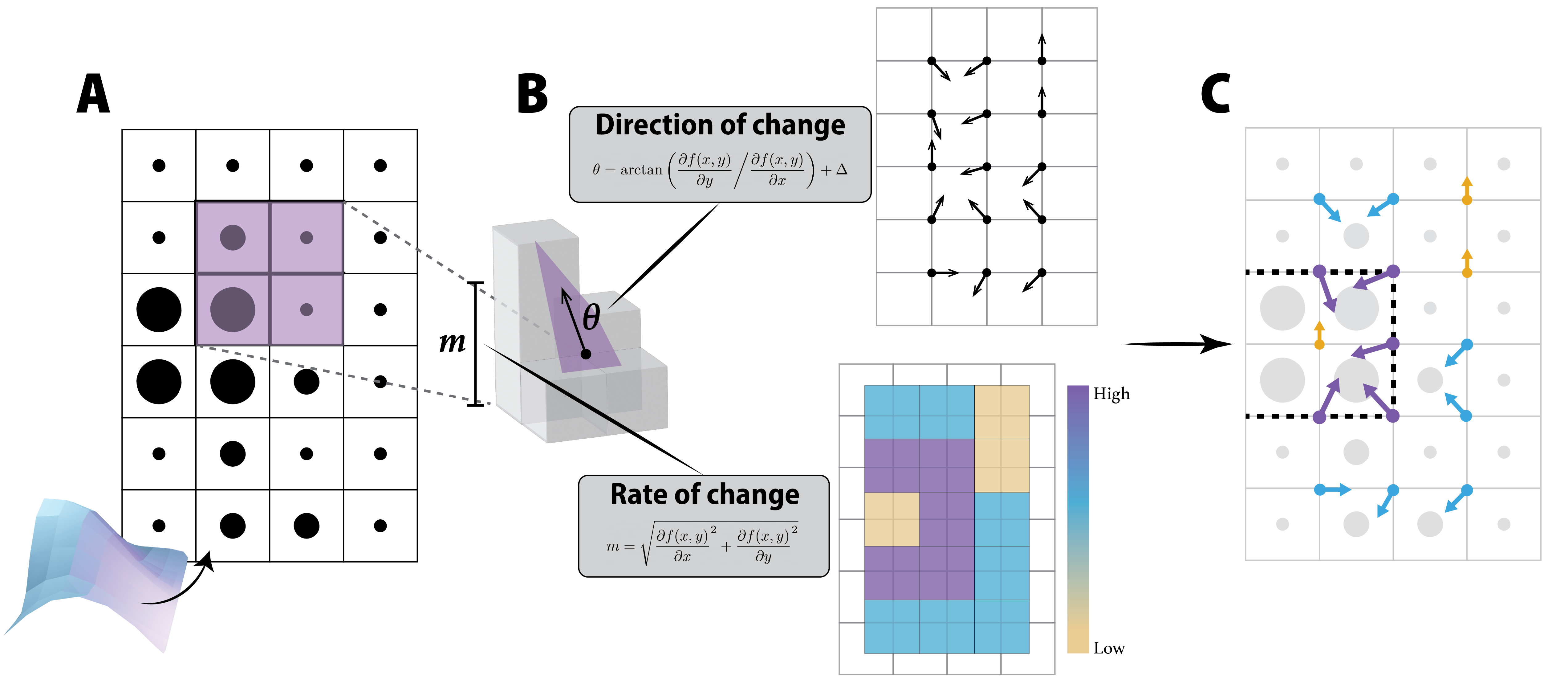
Rate of change

The rate of change (m) can be used to find the zones of rapid change within the geographical area — which, in turn, can be used to identify potential candidate boundaries. The rate of change is calculated as follows:

$$m = \sqrt{\frac{\partial f(x,y)}{\partial x}^2 + \frac{\partial f(x,y)}{\partial y}^2}\qquad{(1)}$$

Where f(x,y) can be expanded as:

f(x,y) = z₁(1−x)(1−y) + z₂x(1−y) + z₃xy + z₄(1−x)y

For convenience the values of the centroid of the ‘search window’ i.e. x and y can be standardised to 0.5 when working with points regularly arranged in space. Additionally, as we are interpolating between points, it should also be noted that the original n * r geographical area will now be an (n−1)(r−1) sized grid (i.e. one less row and one less column of values for the wombled landscape as illustrated in panel C of fig. 1).

When we are working with points that are irregularly arranged within the geographical area it is possible to use triangulation wombling (Fortin 1994, Fortin and Dale 2005, Fortin et al. 2021). Here the approach to wombling has been modified by Fortin (1992) so as to interpolate the plane between the three nearest neighbours (as opposed to the usual 2 × 2 grid). Nearest neighbours are found by using the Delaunay triangulation algorithm (Delaunay 1934) after which the rate of change is still calculated in the same manner as in eq. 1, however as we are now only working with a three-point ‘window’ f(x,y) will be defined as:

f(x,y) = ax + by + c

where

$$\left[ \begin{array}{ccc} a & b & c \end{array} \right] = \left[ {\begin{array}{ccc} x_{1} & y_{1} & 1\\ x_{2} & y_{2} & 1\\ x_{3} & y_{3} & 1\\ \end{array} } \right]^{-1}\cdot \left[ \begin{array}{ccc} z_{1} & z_{2} & z_{3} \end{array} \right]$$

and the x and y co-ordinates of the centroid of the triangle formed by the three points are calculated as follows:

$$ \Big( \frac{x_{1} + x_{2} + x_{3}}{3} \Big), \Big( \frac{y_{1} + y_{2} + y_{3}}{3} \Big) $$

Direction of change

It is also possible to calculate a corresponding direction (θ) for each rate of change (noting that the same equation can be used for both lattice and triangulation wombling). This is calculated as:

$$\theta = \arctan \left( \frac{\partial f(x,y)}{\partial y} \bigg/ \frac{\partial f(x,y)}{\partial x} \right) + \Delta$$

$$\text{where} \quad \Delta = \left\{ \begin{array}{ccc} 0 \degree & \text{if} & \frac{\partial f(x,y)}{\partial x} \geq 0 \\ 180 \degree & \text{if} & \frac{\partial f(x,y)}{\partial x} < 0 \\ \end{array} \right\}$$

This gives the direction of change which, as the name implies, indicates the direction the rate of change is ‘travelling’. The direction of change should be interpreted as wind direction i.e. where the change is coming from and not where it is moving towards. As is the nature of maths when the rate of change is zero it is still possible to calculate a real direction for the non-change — which will be $180\degree$. This means it is possible to think of and use the direction of change independently of calculating boundaries per se and can be used to inform how the landscape is behaving/changing in a more ‘continuous’ way as opposed to discrete zones/boundaries. For example if changes in species richness are more gradual (rate of change is near constant) but the the direction of change is consistently East to West (i.e. $90\degree$) we can still infer that species richness is more or less uniformly increasing in a South-North direction (this is somewhat exemplified in the direction of change landscape of panel B in fig. 1 where the dominant direction of change is East-West).

Candidate boundaries

Detecting boundaries i.e. areas where the angle of the landscape transitions sharply is surprisingly simple. After having calculated the rate of change (m) for the geographical area it is possible to use these values to identify and assign potential boundaries (Oden et al. 1993, Fortin and Drapeau 1995, Fortin and Dale 2005). As large rate of change values are indicative of a steep gradient it stands to reason that these points are indicative of a shift from one state to another i.e. indicative of a boundary. Following the approach outlined in Fortin and Dale (2005) a threshold value (or percentile class) can be set and will determine what proportion of cells will be retained as potential boundaries. For example if using a 0.1 threshold then the highest 10% of points (which are ranked based on m) will be classified as candidate boundaries. Note that points with the same rate of change will be assigned the same rank meaning that more than 10% of the (n−1)(r−1) could potentially be identified as candidate boundary cells. This approach to identifying potential boundary cells is not the sole approach and there are other ways and nuances from which to approach boundary estimation, such as the use of Voronoi tessellations (Oden et al. 1993, Fortin and Drapeau 1995, Matchev et al. 2020).

Methods and features

SpatialBoundaries v0.0.3 implements the Wombling algorithm within the Julia ecosystem and is made available under the permissive MIT license. The source code (along with more extensive documentation) can be found at https://poisotlab.github.io/SpatialBoundaries.jl/. This is an open project and is thus open to contributions. The package itself has two main functions 1) calculate the rate (m) and direction (θ) of change for landscapes for points that are both regularly (i.e. lattice wombling) and irregularly arranged cross space (triangulation wombling) arranged in space using the wombling function (for which layers can also be aggregated using mean), and 2) identifying candidate boundary cells based on a user defined threshold value using the boundaries function. Objects that have been passed through a wombling function are of the Womble abstract type (which has the two sub-types of LatticeWomble and TriangulationWomble). This package is, to the best of our knowledge, the only package to implement the Wombling algorithm within Julia.

Wombling

The wombling function calculates and outputs both the rate (m) and direction (θ; where the direction is denoted from the ‘low’ to the ‘high’ point) of change for a given geographical area. Leveraging the multiple dispatch within Julia this one function will execute either the lattice or triangulation wombling algorithm depending on the structure (spatial referencing) of the input dataset, meaning that it does not need to be user specified. When a matrix of z values is used (where the row and column id’s act as the co-ordinates) the lattice wombling algorithm will be executed and when three vectors (consisting of the co-ordinates (x and y), and z values respectively) the triangulation wombling algorithm is executed. The resulting output object will have two components (m and θ) and will be typed based on the wombling method used. That is a uniform matrix will result in an object of the type LatticeWomble and irregularly arranged points will be of the type TriangulationWomble.

Overall mean wombling value

The mean function calculates the Overall mean wombling value. The methodology stems from the Overall Mean Lattice-Wombling Value (m̄) used by Fortin (1994) in which multiple surfaces (think different z variables) can be overlaid for the purpose of finding the mean rates and directions of change for a composite landscape. The mean rate of change can be defined as the average of m values (for a specific centroid) for the given set of surfaces and the same is done for the direction of change using the θ values. Alongside the mean the standard deviation is also calculated for both the rate and direction of change. Although Fortin (1994) only present this approach for lattice wombled landscapes we have extended the functionality to include both lattice and triangulation wombled types. This is provided that the landscape (i.e. co-ordinates) of the different surfaces are exactly the same. Note here that the original wombling type is retained and the output data will remain either type LatticeWomble or TriangulationWomble.

Boundaries

The boundaries function takes the rate of change (m) of an object of either of the two Womble types (i.e. LatticeWomble or TriangulationWomble), and identifies potential boundary cells based on a user specified threshold (with the default being 0.1). As opposed to selecting only one threshold value we recommend inputting a range of threshold values into the boundaries function to assess how it changes the number of points retained (i.e. boundary cells identified). For example we might see sharp transitions in the number of points that are retained as the threshold value is increased. This inflection point is probably the ideal threshold value to use for boundary selection as a rapid increase in the number of points retained is indicative of a large number of cells with the same rate of change.

Woody areas of the Hawaiian Islands: a wombling example

Below is an example using the various functions within SpatialBoundaries to estimate boundaries for (i.e. patches of) wooded areas on the Southwestern islands of the Hawaiian Islands using landcover data from the EarthEnv project (Tuanmu and Jetz 2014) as well as integrating some functionality from SimpleSDMLayers (Dansereau and Poisot 2021) for easier work with the spatial nature of the input data. The SpatialBoundaries package works really well with SimpleSDMLayers, so that you can (i) apply wombling and boundaries finding to a SimpleSDMLayer object, and (ii) convert the output of a Womble object to a pair of SimpleSDMLayer corresponding to the rate and direction of change.

Because there are four different layers in the EarthEnv database that represent different types of woody cover we will use the overall mean wombling value. As the data are arranged in a matrix i.e. a lattice this example will focus on lattice wombling, however for triangulation wombling the implementation of functions and workflow would look similar with the exception that the input data would be structured differently (as three vectors of x, y, z) and the output data would be typed as TriangulationWomble objects.

using SpatialBoundaries
using SpeciesDistributionToolkit
using CairoMakie
import Plots

Note that the warning about dependencies is a side-effect of loading some functionalities for SimpleSDMLayers as part of SpatialBoundaries, and can safely be ignored.

First we can start by defining the extent of the Southwestern islands of Hawaii, which can be used to restrict the extraction of the various landcover layers from the EarthEnv database. We do the actual database querying using SimpleSDMLayers.

hawaii = (left = -160.2, right = -154.5, bottom = 18.6, top = 22.5)
dataprovider = RasterData(EarthEnv, LandCover)
landcover_classes = SimpleSDMDatasets.layers(dataprovider)
landcover = [SimpleSDMPredictor(dataprovider; layer=class, full=true, hawaii...) for class in landcover_classes]

We can remove all the areas that contain 100% water from the landcover data as our question of interest is restricted to the terrestrial realm. We do this by using the “Open Water” layer to mask over each of the landcover layers individually:

ow_index = findfirst(isequal("Open Water"), landcover_classes)
not_water = landcover[ow_index] .!== 0x64
lc = [mask(not_water, layer) for layer in landcover]

As layers one through four of the EarthEnv data are concerned with data on woody cover (i.e. “Evergreen/Deciduous Needleleaf Trees”, “Evergreen Broadleaf Trees”, “Deciduous Broadleaf Trees”, and “Mixed/Other Trees”) we will work with only these layers. To get a sense of the overall structure of raw landcover components we can sum these four layers and plot the total woody cover for the Southwestern islands (The code for the plot below will give us panel A in fig. 2).

classes_with_trees = findall(contains.(landcover_classes, "Trees"))
tree_lc = convert(Float32, reduce(+, lc[classes_with_trees]))
heatmap(tree_lc; colormap=:linear_kbgyw_5_98_c62_n256)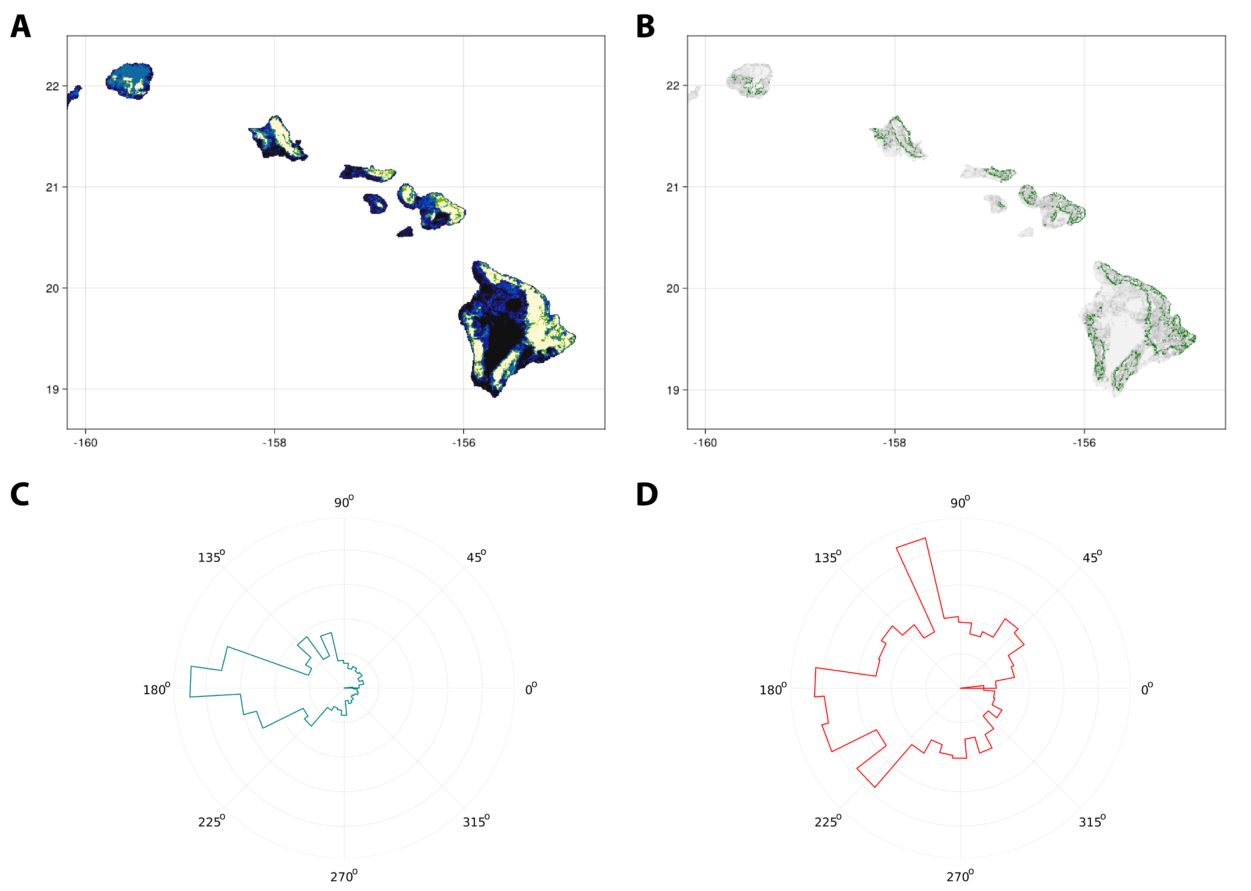

Although we have previously summed the four landcover layers for the actual wombling part we will apply the wombling function to each layer before we calculate the overall mean wombling value. We can broadcast wombling in an element-wise fashion to the four different woody cover layers. This will give as a vector containing four LatticeWomble objects (since the input data was in the form of a matrix).

wombled_layers = wombling.(lc[classes_with_trees])

As we are interested in overall woody cover for Southwestern islands we can take the wombled_layers vector and use them with the mean function to get the overall mean wombling value of the rate and direction of change for woody cover. This will ‘flatten’ the four wombled layers into a single LatticeWomble object.

wombled_mean = mean(wombled_layers)

From the wombled_mean object we can ‘extract’ the layers for both the mean rate and direction of change. For ease of plotting we will also convert these layers to SimpleSDMPredictor type objects. It is also possible to call these matrices directly from the wombled_mean object, which has fields for m (the magnitude of change) and θ (the direction of change).

rate, direction = SimpleSDMPredictor(wombled_mean)

Lastly we can identify candidate boundaries using the boundaries. Here we will use a thresholding value (t) of 0.1 and save these candidate boundary cells as b. Note that we are now working with a SimpleSDMResponse object and this is simply for ease of plotting.

b = similar(rate)
b.grid[boundaries(wombled_mean, 0.1; ignorezero = true)] .= 1.0

In addition to being used to help find candidate boundary cells we can also use this object (b) as masking layer when visualising wombling outputs. In this case we can view the rate layer in a similar fashion to the original landcover layer but by masking it with b we only plot the candidate boundaries (B in fig. 2) i.e. the cells with the top 10% of highest rate of change values. For visualisation we will overlay the identified boundaries (in green) over the rate of change (in levels of grey)

heatmap(rate, colormap=[:grey95, :grey5])
heatmap!(b, colormap=[:transparent, :green])
current_figure()

For this example we will plot the direction of change as radial plots (third and fourth panels in fig. 2) to get an idea of the prominent direction of change. Here we will plot all the direction values from direction for which the rate of change is greater than zero (so as to avoid denoting directions for a slope that does not exist) as well as the direction values from only candidate cells using the same masking principle as what we did for the rate of change. It is of course also possible to forgo the radial plots and plot the direction of change in the same manner as the rate of change should one wish.

Before we plot let us create our two ‘masked layers’. For all direction values for which there is a corresponding rate of change greater than zero we can use rate as a masking layer but first replace all zero values with ‘nothing’. For the candidate boundary cells we can simply mask direction with b as we did for the rate of change.

direction_all = mask(replace(rate, 0 => nothing), direction)

direction_candidate = mask(b, direction)

Because stephist() requires a vector of radians for plotting we must first collect the cells and convert them from degrees to radians. Then we can start by plotting the direction of change of all cells (C in fig. 2).

Plots.stephist(
         deg2rad.(values(direction_all));
         proj=:polar,
         lab="",
         c=:teal,
         nbins = 36,
         yshowaxis=false,
         normalize = false,
         dpi=600)

Followed by plotting the direction of change only for cells that are considered as candidate boundary cells (D in fig. 2).

Plots.stephist(
                deg2rad.(values(direction_candidate));
                proj=:polar,
                lab="",
                c=:red,
                nbins = 36,
                yshowaxis=false,
                normalize = false,
                dpi=600)

Summary

Edge and boundary detection (as well as their delineation) is an important and valuable concept in spatial ecology (Cadenasso et al. 2003) of which wombling serves as an approach that is flexible in its execution (owing to the non-lattice or triangulation capacity of the function) (Fortin 1994, Fortin and Dale 2005) as well as it’s capacity to detect more nuanced landscape changes as opposed to being limited to more abrupt discontinuities such as cliffs/ridges by reducing noise in the landscape (Matchev et al. 2020). Wombling sets us up to answer two questions about the geographic area of interest: at what rate and in which direction does the variable of interest change? This of course has value when it comes to evaluating the variation (or uniformity for that matter) of a suite of ecological variables as well as how they may vary with relation to each other.

SpatialBoundaries.jl provides the toolset with which to implement both lattice and triangulation wombling using the wombling function - multiple dispatch means that the structure of the input dataset will determine exactly which algorithm is implemented. This will simultaneously calculate both the rate and direction of change and if desired multiple sets of different layers of the same geographic area but defined by different z-variables/surfaces can be aggregated and averaged to calculate the overall mean wombling value. Both wombling and mean will return objects of the type Womble of either the sub-type LatticeWomble or TriangulationWomble depending on which method was used. An object of any sub-type Womble can be input into the boundaries function so as to identify cells that can be considered as candidate boundaries based on a user specified threshold.

Acknowledgements: We acknowledge that this study was conducted on land within the traditional unceded territory of the Saint Lawrence Iroquoian, Anishinabewaki, Mohawk, Huron-Wendat, and Omàmiwininiwak nations. TS and TP are funded by a donation from the Courtois Foundation.

References