SDM with maximum entropy
using SpeciesDistributionToolkit
const SDT = SpeciesDistributionToolkit
using PrettyTables
using CairoMakie
In this vignette, we will use the Maxent model (Phillips et al., 2006) to predict the distribution of a bird species. Specifically, we rely on the more modern maxnet version (Phillips et al., 2017).
Model training
There is a vignette outlining the model training pipeline, as well as a use-case on building a model specifically on spatial data. They are good companions to this vignette.
Observations and environmental data
We will collect observations of the Northern Cardinal (Cardinalis cardinalis) for the country of Belize. They are available on GBIF as a DarwinCore archive, which we can download and use directly. The usual Maxent example is the three-toed sloth or the Eucalyptus, but some variety is good for the soul.
records = GBIF.download("10.15468/dl.y8d8yb");
bb = SDT.boundingbox(records; padding = 0.5)
(left = -89.64237, right = -87.62319, bottom = 15.660575999999999, top = 18.954216)We will first grab a series of polygons to define our study area.
borders = getpolygon(PolygonData(NaturalEarth, Countries))
aoi = borders["Belize"]
landmass = clip(borders, bb)
FeatureCollection with 4 features, each with 4 propertiesWe finally get the BioClim variables from CHELSA2, and mask them using the area of interest:
provider = RasterData(CHELSA2, BioClim)
L = SDMLayer{Float32}[SDMLayer(provider; bb..., layer = i) for i in 1:19]
mask!(L, aoi)
19-element Vector{SDMLayer{Float32}}:
🗺️ A 396 × 244 layer (27268 Float32 cells)
🗺️ A 396 × 244 layer (27268 Float32 cells)
🗺️ A 396 × 244 layer (27268 Float32 cells)
🗺️ A 396 × 244 layer (27268 Float32 cells)
🗺️ A 396 × 244 layer (27268 Float32 cells)
🗺️ A 396 × 244 layer (27268 Float32 cells)
🗺️ A 396 × 244 layer (27268 Float32 cells)
🗺️ A 396 × 244 layer (27268 Float32 cells)
🗺️ A 396 × 244 layer (27268 Float32 cells)
🗺️ A 396 × 244 layer (27268 Float32 cells)
🗺️ A 396 × 244 layer (27268 Float32 cells)
🗺️ A 396 × 244 layer (27268 Float32 cells)
🗺️ A 396 × 244 layer (27268 Float32 cells)
🗺️ A 396 × 244 layer (27268 Float32 cells)
🗺️ A 396 × 244 layer (27268 Float32 cells)
🗺️ A 396 × 244 layer (27268 Float32 cells)
🗺️ A 396 × 244 layer (27268 Float32 cells)
🗺️ A 396 × 244 layer (27268 Float32 cells)
🗺️ A 396 × 244 layer (27268 Float32 cells)Pseudo-absences
We start by spatially thinning the observations by mapping them to the predictor layer:
presencelayer = mask(L[1], records)🗺️ A 396 × 244 layer with 27268 Bool cells
Spatial Reference System: +proj=longlat +datum=WGS84 +no_defsWe will now define the area in which we can sample background points, by allowing any pixel that is at least 10km from an observation, but not more than 40km.
background = pseudoabsencemask(BetweenRadius, presencelayer; closer = 10.0, further = 40.0)🗺️ A 396 × 244 layer with 27268 Bool cells
Spatial Reference System: +proj=longlat +datum=WGS84 +no_defsWe finally sample two background points for every cell with at least an observation:
absencelayer = backgroundpoints(background, 2sum(presencelayer))🗺️ A 396 × 244 layer with 27268 Bool cells
Spatial Reference System: +proj=longlat +datum=WGS84 +no_defsPseudo-absences
There are many additional ways to define pseudo-absences, all described in the relevant vignette.
At this point, we have a dataset with all the relevant information, and we are ready to start training the model.
Training and validating the model
Our model will use Maxent for the prediction, and keep the predictor data as they are.
m = SDM(RawData, Maxent, L, presencelayer, absencelayer)❎ RawData → Maxent → P(x) ≥ 0.5 🗺️We can change the hyper-parameters of the model, by allowing product features:
hyperparameters!(classifier(m), :product, true);For cross-validation, we will rely on a series of 10 folds:
folds = kfold(m);Because we do not know whether all variables are relevant, we will select the variables using cross-validation, which will also train the model.
variables!(m, ForwardSelection, folds)☑️ RawData → Maxent → P(x) ≥ 0.504 🗺️Variable selection
There are additional ways to perform variable selection, including by forcing the inclusion of some variables, and they are described in the relevant vignette.
At this point, our Maxent model is entirely trained, and ready to use.
Comparing to another model
It may be a good idea to compare the model with Maxent to another model. We will use logistic regression, and select the variables using the same division of the dataset.
n = SDM(RawData, Logistic, L, presencelayer, absencelayer)
variables!(n, ForwardSelection, folds)
☑️ RawData → Logistic → P(x) ≥ 0.557 🗺️In order to compare the two models, we will cross-validate them (note that we use a different division of the dataset here):
folds = kfold(m);
cv = crossvalidate(m, folds);
cvl = crossvalidate(n, folds);
Finally, we can compare the performance of the two models, using a series of relevant measures:
ms = [mcc, ppv, npv, f1]
M = permutedims([
    m(c) for m in ms, c in [cv.training, cv.validation, cvl.training, cvl.validation]
]);
M = hcat(["Maxent", "", "Logistic", ""], ["Train.", "Val.", "Train.", "Val."], M);
These are the results:
pretty_table(
    M;
    alignment = [:l, :l, :c, :c, :c, :c],
    backend = :markdown,
    column_labels = [""; "Dataset"; string.(ms)],
    formatters = [fmt__printf("%5.3f", [3, 4, 5, 6])],
)| Dataset | mcc | ppv | npv | f1 | |
|---|---|---|---|---|---|
| Maxent | Train. | 0.855 | 0.971 | 0.919 | 0.897 |
| Val. | 0.855 | 0.971 | 0.919 | 0.897 | |
| Logistic | Train. | 0.938 | 0.965 | 0.976 | 0.959 |
| Val. | 0.935 | 0.964 | 0.975 | 0.957 |
Maxent is not as good as logistic regression for this problem (with the exception of the ability to detect positives, which is slightly better). But because this is the Maxent vignette, we will nonetheless keep going with it, for the sake of illustration.
Maxent results
We will first map the prediction of the maxent model (and compare it to the logistic prediction).
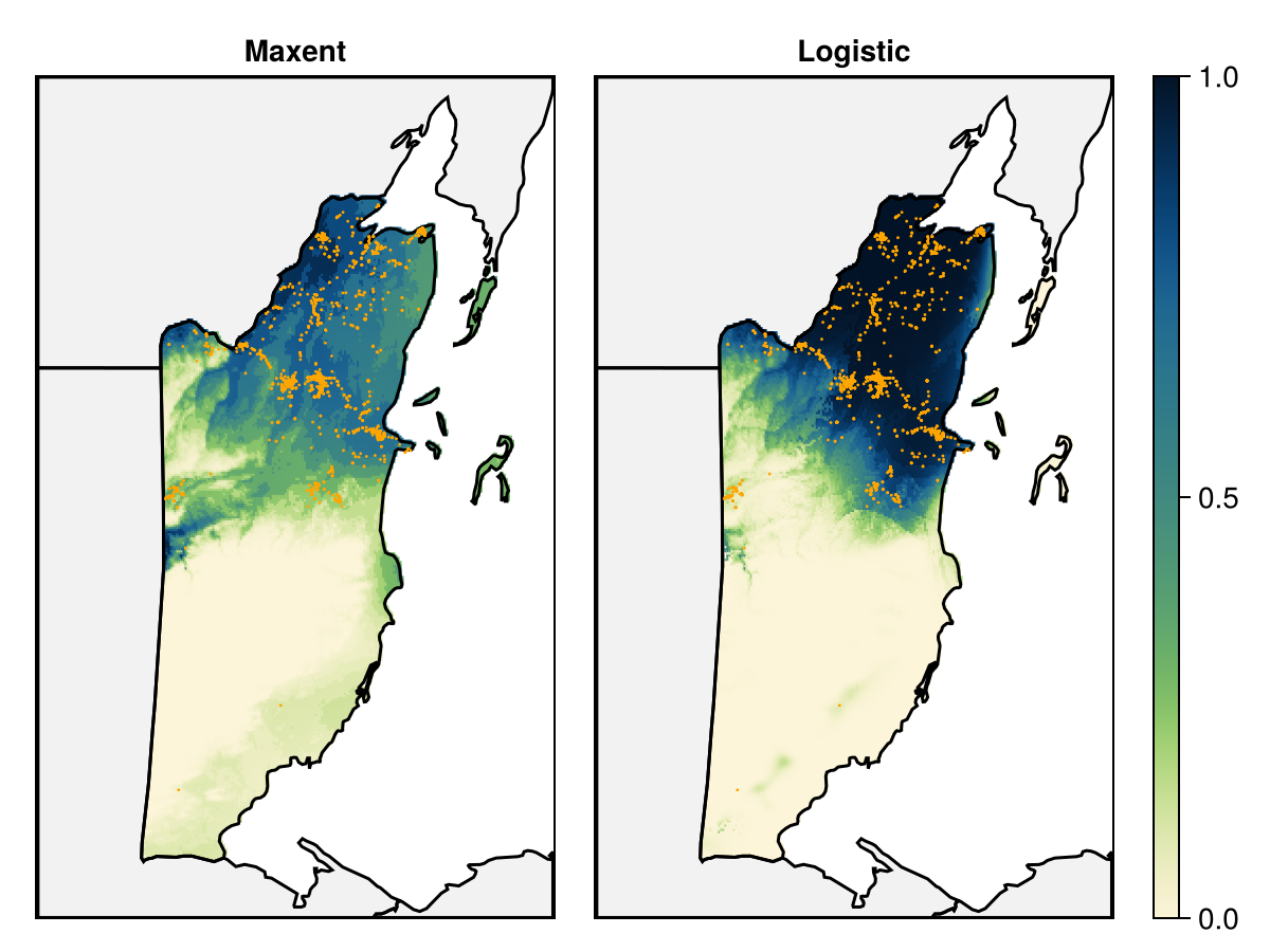
Code for the figure
f = Figure()
ax = Axis(f[1, 1]; aspect = DataAspect(), title = "Maxent")
ax2 = Axis(f[1, 2]; aspect = DataAspect(), title = "Logistic")
for a in [ax, ax2]
    poly!(a, landmass; color = :grey95)
end
hm = heatmap!(
    ax,
    predict(m, L; threshold = false);
    colormap = Reverse(:navia),
    colorrange = (0, 1),
)
heatmap!(
    ax2,
    predict(n, L; threshold = false);
    colormap = Reverse(:navia),
    colorrange = (0, 1),
)
for a in [ax, ax2]
    lines!(a, landmass; color = :black)
    scatter!(a, records; color = :orange, markersize = 2)
    tightlimits!(a)
    hidedecorations!(a)
end
Colorbar(f[1, 3], hm)
We can look at the partial response to the variable that was included first in the model, in order to understand how it translates into a high predicted value:
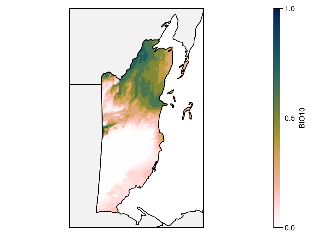
Code for the figure
f = Figure()
ax = Axis(f[1, 1]; aspect = DataAspect())
poly!(ax, landmass; color = :grey95)
hm = heatmap!(
    ax,
    partialresponse(m, L, first(variables(m)); threshold = false);
    colormap = Reverse(:batlowW),
    colorrange = (0, 1),
)
lines!(ax, landmass; color = :black)
tightlimits!(ax)
hidedecorations!(ax)
Colorbar(f[1, 2], hm; label = layers(provider)[first(variables(m))])
We can also look at the effect of this variable's value on the average model prediction using Shapley Monte-Carlo values.
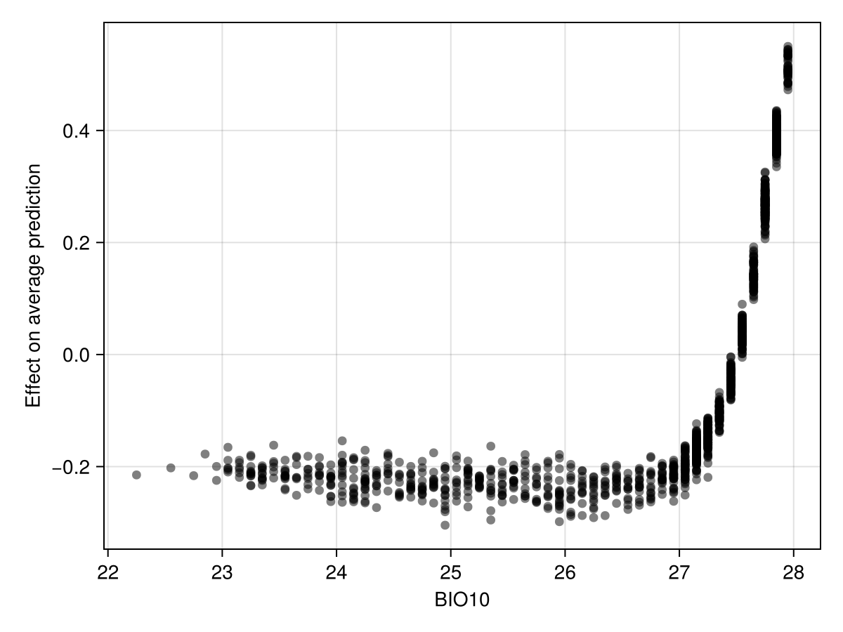
Code for the figure
f = Figure()
ax = Axis(
    f[1, 1];
    xlabel = layers(provider)[first(variables(m))],
    ylabel = "Effect on average prediction",
)
scatter!(
    ax,
    features(m, first(variables(m))),
    explain(m, first(variables(m)); threshold = false);
    color = (:black, 0.5),
)
This shows that the presence of the species becomes more likely to be predicted when the value of this variable is higher.
Related documentation
SDeMo.Maxent Type
MaxentMaximum entropy, using the Maxnet.jl package.
Different types of features can be included/excluded using the hyperparamters! function, with :linear and :categorical (default to true), as well as :hinge and :product (default to false). If all four responses are set to false, the default decision rule based on number of presences will be applied.
The :regularization hyper-parameter is a scalar (defaults to 1.0) for the inclusion of new features.
The :linkfunction is used at prediction time, and the value of :default is C log-log link. Other values are :logit, :log, and :identity.
SDeMo.hyperparameters! Function
hyperparameters!(tr::HasHyperParams, hp::Symbol, val)Sets the hyper-parameters for a transformer or a classifier
sourceSDeMo.crossvalidate Function
crossvalidate(sdm, folds; thr = nothing, kwargs...)Performs cross-validation on a model, given a vector of tuples representing the data splits. The threshold can be fixed through the thr keyword arguments. All other keywords are passed to the train! method.
This method returns two vectors of ConfusionMatrix, with the confusion matrix for each set of validation data first, and the confusion matrix for the training data second.
crossvalidate(sdm::T, args...; kwargs...) where {T <: AbstractSDM}Performs cross-validation using 10-fold validation as a default. Called when crossvalidate is used without a folds second argument.
References
Phillips, S. J.; Anderson, R. P.; Dudík, M.; Schapire, R. E. and Blair, M. E. (2017). Opening the black box: an open-source release of Maxent. Ecography 40, 887–893. Publisher: Wiley.
Phillips, S. J.; Anderson, R. P. and Schapire, R. E. (2006). Maximum entropy modeling of species geographic distributions. Ecological Modelling 190, 231–259. Accessed on Aug 19, 2025.