Boosting and calibrating a probabilistic classifier
In this vignette, we will see how we can use AdaBoost to turn a mediocre model into a less mediocre one.
using SpeciesDistributionToolkit
const SDT = SpeciesDistributionToolkit
using CairoMakie
Data preparation
We will use the demonstration data, and setup a simple decision tree. We will refine its hyper-parameters later on.
aoi = getpolygon(PolygonData(OpenStreetMap, Places); place = "Corse")
provider = RasterData(CHELSA2, BioClim)
L = SDMLayer{Float32}[
    SDMLayer(
        provider;
        layer = x,
        SDT.boundingbox(aoi)...,
    ) for x in 1:19
];
mask!(L, aoi)
19-element Vector{SDMLayer{Float32}}:
🗺️ A 205 × 124 layer (13685 Float32 cells)
🗺️ A 205 × 124 layer (13685 Float32 cells)
🗺️ A 205 × 124 layer (13685 Float32 cells)
🗺️ A 205 × 124 layer (13685 Float32 cells)
🗺️ A 205 × 124 layer (13685 Float32 cells)
🗺️ A 205 × 124 layer (13685 Float32 cells)
🗺️ A 205 × 124 layer (13685 Float32 cells)
🗺️ A 205 × 124 layer (13685 Float32 cells)
🗺️ A 205 × 124 layer (13685 Float32 cells)
🗺️ A 205 × 124 layer (13685 Float32 cells)
🗺️ A 205 × 124 layer (13685 Float32 cells)
🗺️ A 205 × 124 layer (13685 Float32 cells)
🗺️ A 205 × 124 layer (13685 Float32 cells)
🗺️ A 205 × 124 layer (13685 Float32 cells)
🗺️ A 205 × 124 layer (13685 Float32 cells)
🗺️ A 205 × 124 layer (13685 Float32 cells)
🗺️ A 205 × 124 layer (13685 Float32 cells)
🗺️ A 205 × 124 layer (13685 Float32 cells)
🗺️ A 205 × 124 layer (13685 Float32 cells)Fundamental of model use
There is a vignette on declaring, training, and using models, which covers a lot of ground that will help make sense of the syntax.
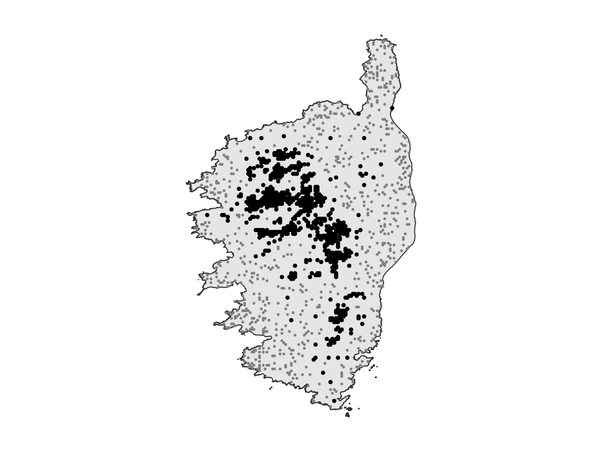
model = SDM(RawData, DecisionTree, SDeMo.__demodata()...)❎ RawData → DecisionTree → P(x) ≥ 0.5 🗺️This is the dataset we start from:
Code for the figure
fig = Figure()
ax = Axis(fig[1, 1]; aspect = DataAspect())
poly!(ax, aoi; color = :grey90, strokewidth = 1, strokecolor = :grey20)
scatter!(ax, presences(model); color = :black, markersize = 6)
scatter!(ax, absences(model); color = :grey50, markersize = 4)
hidedecorations!(ax)
hidespines!(ax)
Initial model
Before building the boosting model, we need to construct a weak learner.
The BIOCLIM model (Booth et al., 2014) is one of the first SDM that was ever published. Because it is a climate envelope model (locations within the extrema of environmental variables for observed presences are assumed suitable, more or less), it does not usually give really good predictions. BIOCLIM underfits, and for this reason it is also a good candidate for boosting. Naive Bayes classifiers are similarly suitable for AdaBoost: they tend to achieve a good enough performance in aggregate, but due to the way they learn from the data, they rarely excel at any single prediction.
The traditional lore is that AdaBoost should be used only with really weak classifiers, but Wyner et al. (2017) have convincing arguments in favor of treating it more like a random forest, by showing that it also works with comparatively stronger learners. In keeping with this idea, we will train a moderately deep tree as our base classifier.
hyperparameters!(classifier(model), :maxdepth, 4)
hyperparameters!(classifier(model), :maxnodes, 4)
DecisionTree(SDeMo.DecisionNode(nothing, nothing, nothing, 0, 0.0, 0.5, false), 4, 4)Decision stumps
using a maximum depth of 1 and a maximum nodes of 2 would turn this model into a decision stump, which is a very interesting type of classifier that relies on stacking many mediocre predictions into an often surprisingly good one.
This tree is not quite a decision stump (a one-node tree), but they are relatively small, so a single one of them is unlikely to give a good prediction. We can train the model and generate the initial prediction:
train!(model)
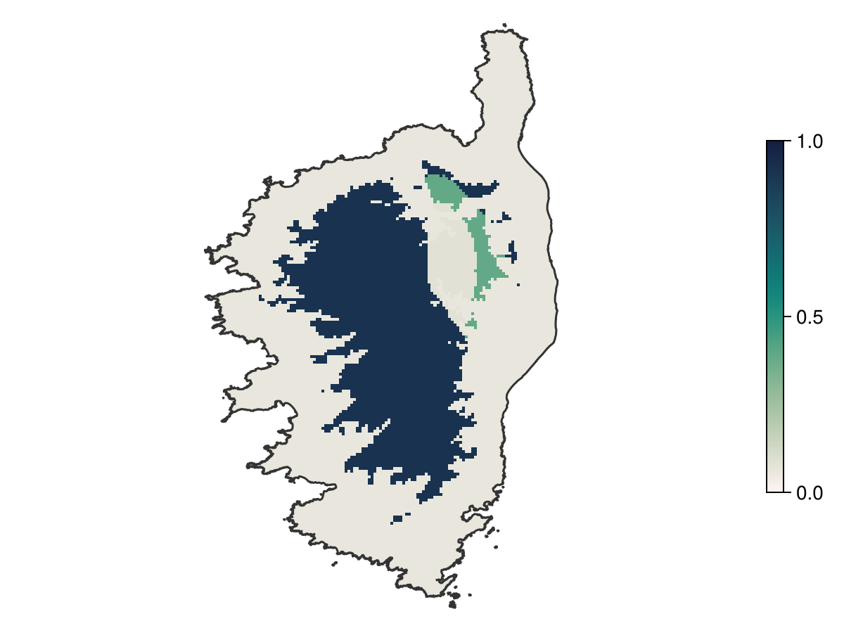
prd = predict(model, L; threshold = false)🗺️ A 205 × 124 layer with 13685 Float64 cells
Spatial Reference System: +proj=longlat +datum=WGS84 +no_defsAs expected, although it roughly identifies the range of the species, it is not doing a spectacular job at it. This model is a good candidate for boosting.
Code for the figure
f = Figure()
ax = Axis(f[1,1]; aspect=DataAspect())
hm = heatmap!(ax, prd; colormap = :tempo, colorrange = (0, 1))
lines!(ax, aoi; color = :grey20)
hidedecorations!(ax)
hidespines!(ax)
Colorbar(f[1, 2], hm; height = Relative(0.6))
Boosting
To train this model using the AdaBoost algorithm, we wrap it into an AdaBoost object, and specify the number of iterations (how many learners we want to train). The default is 50.
bst = AdaBoost(model; iterations = 60)AdaBoost {RawData → DecisionTree → P(x) ≥ 0.393} × 60 iterationsWe will decrease the learning rate of this model a little bit:
hyperparameters!(bst, :η, 0.9)AdaBoost {RawData → DecisionTree → P(x) ≥ 0.393} × 60 iterationsTraining the model is done in the exact same way as other SDeMo models, with one important exception. AdaBoost uses the predicted class (presence/absence) internally, so we will always train learners to return a thresholded prediction. For this reason, even it the threshold argument is used, it will be ignored during training.
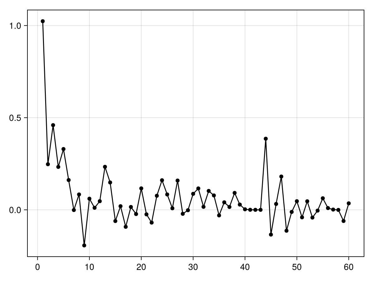
train!(bst)AdaBoost {RawData → DecisionTree → P(x) ≥ 0.393} × 60 iterationsWe can look at the weight (i.e. how much a weak learner is trusted during the final prediction) over time. It should decrease, and more than that, it should ideally decrease fast (exponentially). Some learners may have a negative weight, which means that they are consistently wrong. These are counted by flipping their prediction in the final recommendation.
Code for the figure
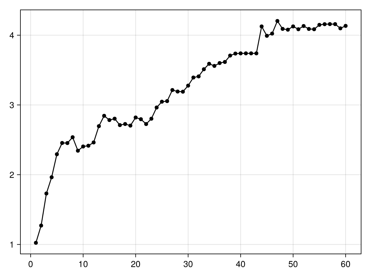
scatterlines(bst.weights; color = :black)Models with a weight of 0 are not contributing new information to the boosted model. These are expected to become increasingly common at later iterations, so it is a good idea to examine the cumulative weights to see whether we get close to a plateau.
Code for the figure
scatterlines(cumsum(bst.weights); color = :black)This is close enough. We can now apply this model to the bioclimatic variables:
brd = predict(bst, L; threshold = false)🗺️ A 205 × 124 layer with 13685 Float64 cells
Spatial Reference System: +proj=longlat +datum=WGS84 +no_defsThis gives the following map:
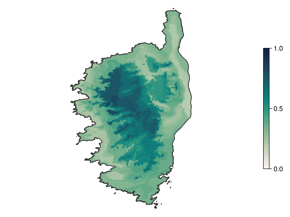
Code for the figure
f = Figure()
ax = Axis(f[1,1]; aspect=DataAspect())
hm = heatmap!(ax, brd; colormap = :tempo, colorrange = (0, 1))
lines!(ax, aoi; color = :grey20)
hidedecorations!(ax)
hidespines!(ax)
Colorbar(f[1, 2], hm; height = Relative(0.6))
Calibration
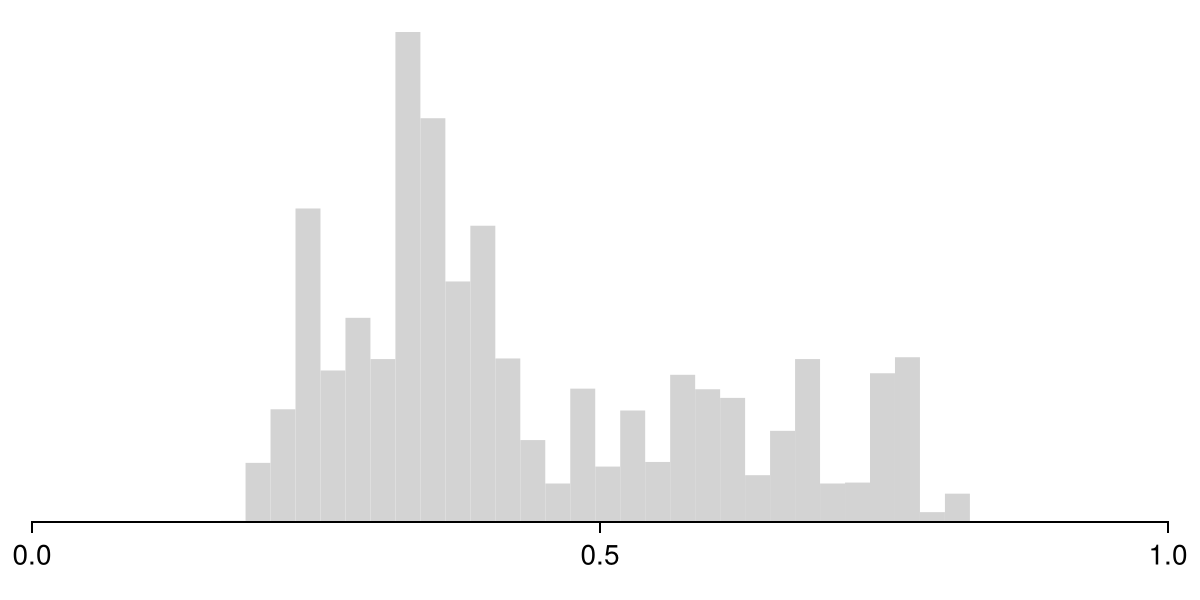
The scores returned by the boosted model are not calibrated probabilities, so they are centered on 0.5, but have typically low variance. This can be explained by the fact that each component models tends to make one-sided errors near 0 and 1, wich accumulate with more models over time. This problem is typically more serious when adding multiple classifiers together, as with bagging and boosting. Some classifiers tend to exagerate the proportion of extreme values (Naive Bayes classifiers, for example), some others tend to create peaks near values slightly above 0 and below 1 (tree-based methods), while methods like logistic regression typically do a fair job at predicting probabilities.
The type of bias that a classifier accumulates is usually pretty obvious from looking at the histogram of the results:
Code for the figure
f = Figure(; size = (600, 300))
ax = Axis(f[1, 1]; xlabel = "Predicted score")
hist!(ax, brd; color = :lightgrey, bins = 30)
hideydecorations!(ax)
hidexdecorations!(ax; ticks = false, ticklabels = false)
hidespines!(ax, :l)
hidespines!(ax, :r)
hidespines!(ax, :t)
xlims!(ax, 0, 1)
tightlimits!(ax)
Here, we see that the predictions are starting to cluster away from 0 and 1, and converge onto about one half. This is not a problem when thinking about the species range, because the thresholding will account for this; but it is a problem when thinking about the predicted score.
We can also look at the reliability curve for this model. The reliability curve divides the predictions into bins, and compares the average score on the training data to the proportion of events in the training data. When these two quantities are almost equal, the score outputed by the model is a good prediction of the probability of the event.

Code for the figure
f = Figure()
ax = Axis(
    f[1, 1];
    aspect = 1,
    xlabel = "Average predicted probability",
    ylabel = "Average empirical probability",
)
lines!(ax, [0, 1], [0, 1]; color = :grey, linestyle = :dash)
xlims!(ax, 0, 1)
ylims!(ax, 0, 1)
scatterlines!(ax, SDeMo.reliability(bst)...; color = :black, label = "Raw scores")
Based on the reliability curve, it is clear that the model outputs are not probabilities; otherwise, they would lay on the 1:1 line. In order to turn these scores into a value that are closer to probabilities, we can estimate calibration parameters for this model:
C = calibrate(bst)PlattCalibration(-8.763135276226246, 4.4798401313050595)This step uses the Platt (1999) scaling approach, where the outputs from the model are regressed against the true class probabilities, to attempt to bring the model prediction more in line with true probabilities (Niculescu-Mizil and Caruana, 2005). Internally, the package uses the fast and robust algorithm of Lin et al. (2007).
These parameters can be turned into a correction function:
f = correct(C)#correct##0 (generic function with 1 method)It is a good idea to check that the calibration function is indeed bringing us closer to the 1:1 line, which is to say that it provides us with a score that is closer to a true probability.
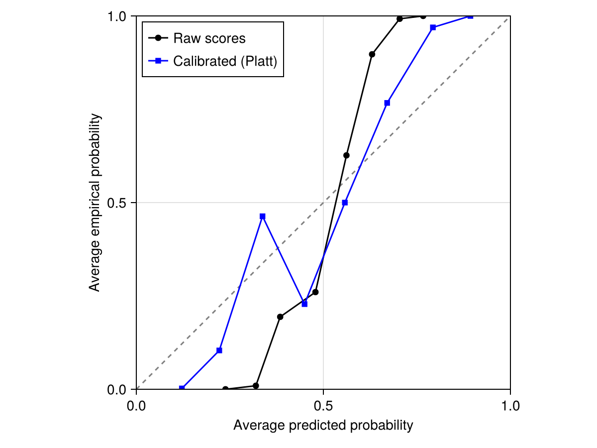
Code for the figure
scatterlines!(
    ax,
    SDeMo.reliability(bst; link = f)...;
    color = :blue,
    marker = :rect,
    label = "Calibrated (Platt)",
)
axislegend(ax; position = :lt)
This calibration function is not quite right for this problem, so we can switch to the more flexible method of isotonic calibration:
C = calibrate(IsotonicCalibration, bst)
calfunc = correct(C)
#correct##0 (generic function with 1 method)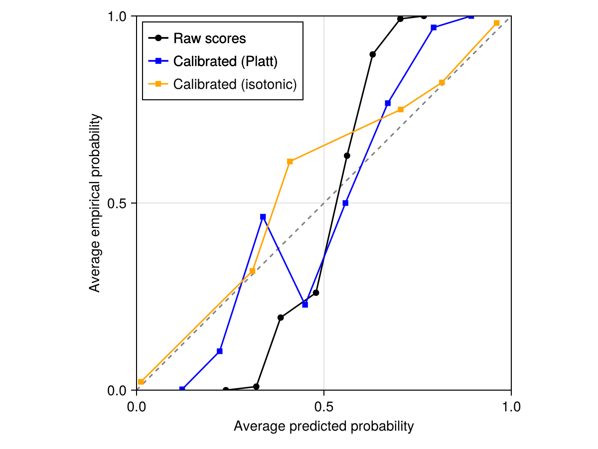
Code for the figure
scatterlines!(
    ax,
    SDeMo.reliability(bst; link = calfunc)...;
    color = :orange,
    marker = :rect,
    label = "Calibrated (isotonic)",
)
axislegend(ax; position = :lt)
This gives a much better result, and so we will use this calibration function to return the probability prediction.
Predicting probabilities
Of course the calibration function can (like any other function) be applied to a layer, so we can now use AdaBoost to estimate the probability of species presence. Dormann (2020) has several strong arguments in favor of this approach.
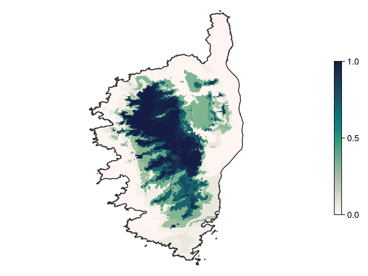
Code for the figure
f = Figure()
ax = Axis(f[1,1]; aspect=DataAspect())
hm = heatmap!(ax, calfunc.(brd); colormap = :tempo, colorrange = (0, 1))
lines!(ax, aoi; color = :grey20)
hidedecorations!(ax)
hidespines!(ax)
Colorbar(f[1, 2], hm; height = Relative(0.6))
Note that the calibration is not required to obtain a binary map, as the transformation applied to the scores is monotonous. For this reason, the AdaBoost function will internally work on the raw scores, and turn them into binary predictions using thresholding.
The default threshold for AdaBoost is 0.5, which is explained by the fact that the final decision step is a weighted voting based on the sum of all weak learners. We can get the predicted range under both models:
sdm_range = predict(model, L)
bst_range = predict(bst, L)
🗺️ A 205 × 124 layer with 13685 Bool cells
Spatial Reference System: +proj=longlat +datum=WGS84 +no_defsWe now plot the difference, where the areas gained by boosting are in green, and the areas lost by boosting are in light grey. The part of the range that is conserved is in black.
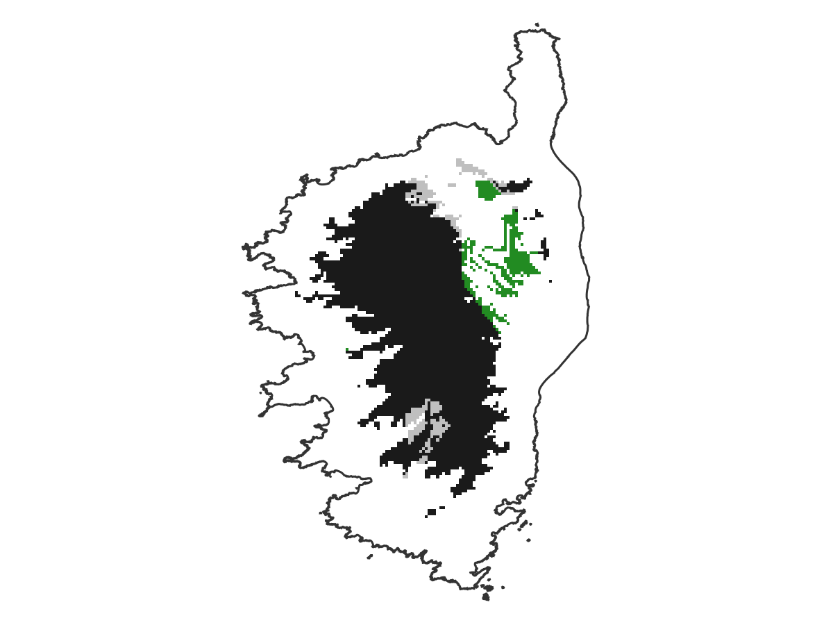
Code for the figure
fg, ax, pl = heatmap(
    gainloss(sdm_range, bst_range);
    colormap = [:forestgreen, :grey10, :grey75],
    colorrange = (-1, 1),
)
ax.aspect = DataAspect()
hidedecorations!(ax)
hidespines!(ax)
lines!(ax, aoi; color = :grey20)
Related documentation
SDeMo.AdaBoost Type
AdaBoost <: AbstractBoostedSDMA type for AdaBoost that contains the model, a vector of learners, a vector of learner weights, a number of boosting iterations, and the weights w of each point.
Note that this type uses training by re-sampling data according to their weights, as opposed to re-training on all samples and weighting internally. Some learners may have negative weights, in which case their predictions are flipped at prediction time.
The learning rate η defaults to one, but can be lowered to improve stability / prevent over-fitting. The learning rate must be larger than 0, and decreasing it should lead to a larger number of iterations.
SDeMo.calibrate Function
calibration(sdm::T; kwargs...)Returns a function for model calibration, using Platt scaling, optimized with the Newton method. The returned function can be applied to a model output.
sourcecalibrate(::Type{IsotonicCalibration}, sdm::T; bins=25, kwargs...)Returns the isotonic calibration result for a given SDM. Isotonic regression is done using the bin membership as a weight, which gives less importance to bins with a lower membership.
sourceSDeMo.correct Function
correct(cal::AbstractCalibration)Returns a function that gives a probability given a calibration result.
sourcecorrect(cal::Vector{<:AbstractCalibration})Returns a function that gives the average of probabilities from a vector of calibration results. This is used when bootstrapping or cross-validating probabilities using a pre-trained model.
sourceSDeMo.reliability Function
reliability(yhat, y; bins=9)Returns a binned reliability curve for a series of predicted quantitative scores and a series of truth values.
sourcereliability(sdm::AbstractSDM, link::Function=identity; bins=9, kwargs...)Returns a binned reliability curve for a trained model, where the raw scores are transformed with a specified link function (which defaults to identity). Keyword arguments other than bins are passed to predict.
References
Booth, T. H.; Nix, H. A.; Busby, J. R. and Hutchinson, M. F. (2014), bioclim: the first species distribution modelling package, its early applications and relevance to most current MaxEnt studies. Diversity & distributions 20, 1–9. Publisher: Wiley.
Dormann, C. F. (2020). Calibration of probability predictions from machine‐learning and statistical models. Global ecology and biogeography: a journal of macroecology 29, 760–765. Publisher: Wiley.
Lin, H.-T.; Lin, C.-J. and Weng, R. C. (2007). A note on Platt’s probabilistic outputs for support vector machines. Machine learning 68, 267–276. Publisher: Springer Science and Business Media LLC.
Niculescu-Mizil, A. and Caruana, R. (2005). Obtaining calibrated probabilities from boosting. In: Proceedings of the twenty-first conference on uncertainty in artificial intelligence, UAI'05 (AUAI Press, Arlington, Virginia, USA); pp. 413–420, tex.venue: Edinburgh, Scotland.
Platt, J. (1999). Probabilistic outputs for support vector machines and comparisons to regularized likelihood methods. In: Advances in large margin classifiers, edited by Smola, A. J.; Bartlett, P.; Schölkopf, B. and Schuurmans, D. (MIT Press, Cambridge).
Wyner, A. J.; Olson, M.; Bleich, J. and Mease, D. (2017). Explaining the success of adaboost and random forests as interpolating classifiers. Journal of Machine Learning Research 18, 1558–1590. Publisher: JMLR.org.