Shift and rotate
In this tutorial, we will apply the "Shift and Rotate" technique (Ridder et al., 2024) to generate realistic maps of predictors to provide a null sample for the performance of an SDM. We will also look at the quantile mapping function, which ensures that the null sample has the exact same distribution of values compared to the original data.
using SpeciesDistributionToolkit
const SDT = SpeciesDistributionToolkit
using PrettyTables
using CairoMakie
We will get some occurrences about the observations of Cardinalis cardinalis in Belize, which we used in the Maxent vignette.
Model training
There is a vignette outlining the model training pipeline, as well as a use-case on building a model specifically on spatial data. They are good companions to this vignette.
records = GBIF.download("10.15468/dl.y8d8yb");
extent = SDT.boundingbox(records; padding = 3.5)
(left = -92.64237, right = -84.62319, bottom = 12.660575999999999, top = 21.954216)We will first grab a series of polygons to define our study area. We get a polygon for the country borders, and then a second polygon for the landmass, which we will use as the background of our maps.
aoi = getpolygon(PolygonData(NaturalEarth, Countries))["Belize"]
land = getpolygon(PolygonData(NaturalEarth, Land))
landmass = clip(land, extent)
FeatureCollection with 5 features, each with 0 propertiesTo train the model, we will collect all 19 BioClim variables from CHELSA2, and mask them to the landmass we have selected before.
provider = RasterData(CHELSA2, BioClim)
L = SDMLayer{Float32}[SDMLayer(provider; extent..., layer = i) for i in 1:19]
mask!(L, landmass)
19-element Vector{SDMLayer{Float32}}:
🗺️ A 1116 × 964 layer (595407 Float32 cells)
🗺️ A 1116 × 964 layer (595407 Float32 cells)
🗺️ A 1116 × 964 layer (595407 Float32 cells)
🗺️ A 1116 × 964 layer (595407 Float32 cells)
🗺️ A 1116 × 964 layer (595407 Float32 cells)
🗺️ A 1116 × 964 layer (595407 Float32 cells)
🗺️ A 1116 × 964 layer (595407 Float32 cells)
🗺️ A 1116 × 964 layer (595407 Float32 cells)
🗺️ A 1116 × 964 layer (595407 Float32 cells)
🗺️ A 1116 × 964 layer (595407 Float32 cells)
🗺️ A 1116 × 964 layer (595407 Float32 cells)
🗺️ A 1116 × 964 layer (595407 Float32 cells)
🗺️ A 1116 × 964 layer (595407 Float32 cells)
🗺️ A 1116 × 964 layer (595407 Float32 cells)
🗺️ A 1116 × 964 layer (595407 Float32 cells)
🗺️ A 1116 × 964 layer (595407 Float32 cells)
🗺️ A 1116 × 964 layer (595407 Float32 cells)
🗺️ A 1116 × 964 layer (595407 Float32 cells)
🗺️ A 1116 × 964 layer (595407 Float32 cells)Note that are not masking the layer to the area of interest (Belize, the country for which we have data), because we will construct null layers from the value of predictors within the larger region. For this reason, it is very important that all the relevant pixels in the larger region have a value.
Layer interpolation
In order to facilitate the search for rotation parameters, it is a good idea to downscale the layer a little.
We start by picking the first layer, and make a copy of it.
T = copy(first(L))🗺️ A 1116 × 964 layer with 595407 Float32 cells
Spatial Reference System: +proj=longlat +datum=WGS84 +no_defsWe will interpolate it so that each cell is about 25 times as large as before, and has the same projection as the original layer.
NS = ceil.(Int, size(T) ./ 5)
P = interpolate(T; dest = T.crs, newsize = NS)
🗺️ A 224 × 193 layer with 23828 Float32 cells
Spatial Reference System: +proj=longlat +datum=WGS84 +no_defsAt this point, we can collect the actual area that we want to replace with shifted and rotated values:
C = trim(mask(P, aoi))🗺️ A 62 × 35 layer with 1071 Float32 cells
Spatial Reference System: +proj=longlat +datum=WGS84 +no_defsfigure Full area
f = Figure()
ax = Axis(f[1, 1]; aspect = DataAspect())
heatmap!(ax, P; colormap = :batlowW, alpha = 0.5, colorrange = extrema(P))
lines!(ax, landmass; color = :grey50)
hm = heatmap!(ax, C; colormap = :batlowW, colorrange = extrema(P))
lines!(ax, aoi; color = :black)
Colorbar(f[1, 2], hm; label = "Average temperature")
Finding a rotation
With the two layers, we will now attempt to identify a shift and a rotation. Conceputally, we are attempting to figure out how we can rotate the Earth underneath our layer of interest, both across the latitude and longitude axes, and also along the axis that goes through the center of the layer, while keeping all the cells in the layer having a value.
θ = findrotation(C, P)(-2.515342275199485, -1.0683269566655036, -89.08240785776358)This output represents the rotation as a shift in latitude and longitude, and then a rotation around the axis. It is returned as a tuple, which can be passed to the rotator closure, which handles the actual rotation:
𝑹 = rotator(θ...)SimpleSDMLayers.var"#shiftlongitudes##0#shiftlongitudes##1"{Float64}(-2.515342275199485) ∘ SimpleSDMLayers.var"#shiftlatitudes##0#shiftlatitudes##1"{Float64}(-1.0683269566655036) ∘ SimpleSDMLayers.var"#localrotation##0#localrotation##1"{Float64}(-89.08240785776358)Order of operations
The shift in latitude and longitude can be done in any order, but the rotation is done last. Internally, the functions will always perform these steps in the same order.
The next figure shows the original layer, as well as the coordinates of the points from which its replacement values will be drawn.
figure Full area with rotation
f = Figure()
ax = Axis(f[1, 1]; aspect = DataAspect())
hm = heatmap!(ax, P; colormap = :batlowW, alpha = 0.4)
lines!(ax, landmass; color = :grey50)
poly!(ax, aoi; color = :orange, alpha = 0.5)
lines!(ax, aoi; color = :orange)
scatter!(ax, 𝑹(lonlat(C)); color = :black, markersize = 4, alpha = 0.5)
Colorbar(f[1, 2], hm; label = "Average temperature")
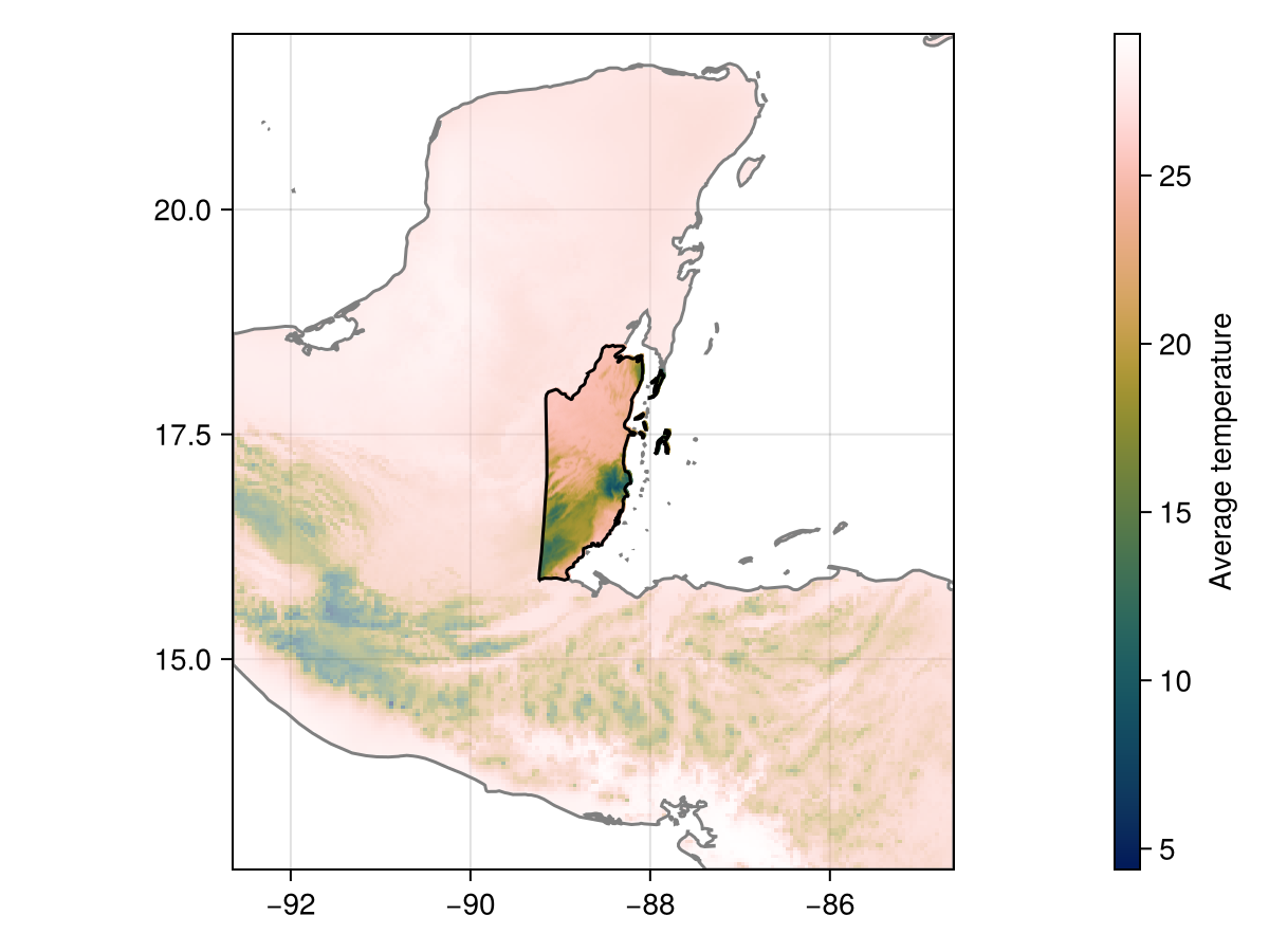
This rotation function can then be applied to the shiftandrotate function, in order to create a modified version of the original layer:
Y = shiftandrotate(C, P, 𝑹)🗺️ A 62 × 35 layer with 1071 Float32 cells
Spatial Reference System: +proj=longlat +datum=WGS84 +no_defs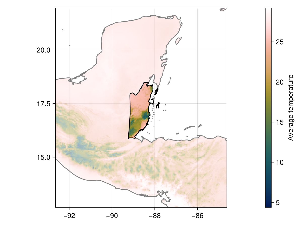
Code for the figure
f = Figure()
ax = Axis(f[1, 1]; aspect = DataAspect())
heatmap!(ax, P; colormap = :batlowW, alpha = 0.4)
lines!(ax, landmass; color = :grey50)
hm = heatmap!(ax, Y; colormap = :batlowW, colorrange = extrema(P))
lines!(ax, aoi; color = :black)
Colorbar(f[1, 2], hm; label = "Average temperature")
Shifting and rotating the layers
We can now apply this transformation to the original (full resolution) data. We will start by trimming the layers to the extent of the area of interest:
X = trim.(mask(L, aoi));We will use these vectors to train the reference species distribution model. We now generate the shifted and rotated version:
M = shiftandrotate(X, L, 𝑹);We can check the version of the shifted and rotated layer in its full resolution:
Code for the figure
f = Figure()
ax = Axis(f[1, 1]; aspect = DataAspect())
heatmap!(ax, P; colormap = :batlowW, alpha = 0.5)
lines!(ax, landmass; color = :grey50)
hm = heatmap!(ax, M[1]; colormap = :batlowW, colorrange = extrema(P))
lines!(ax, aoi; color = :black)
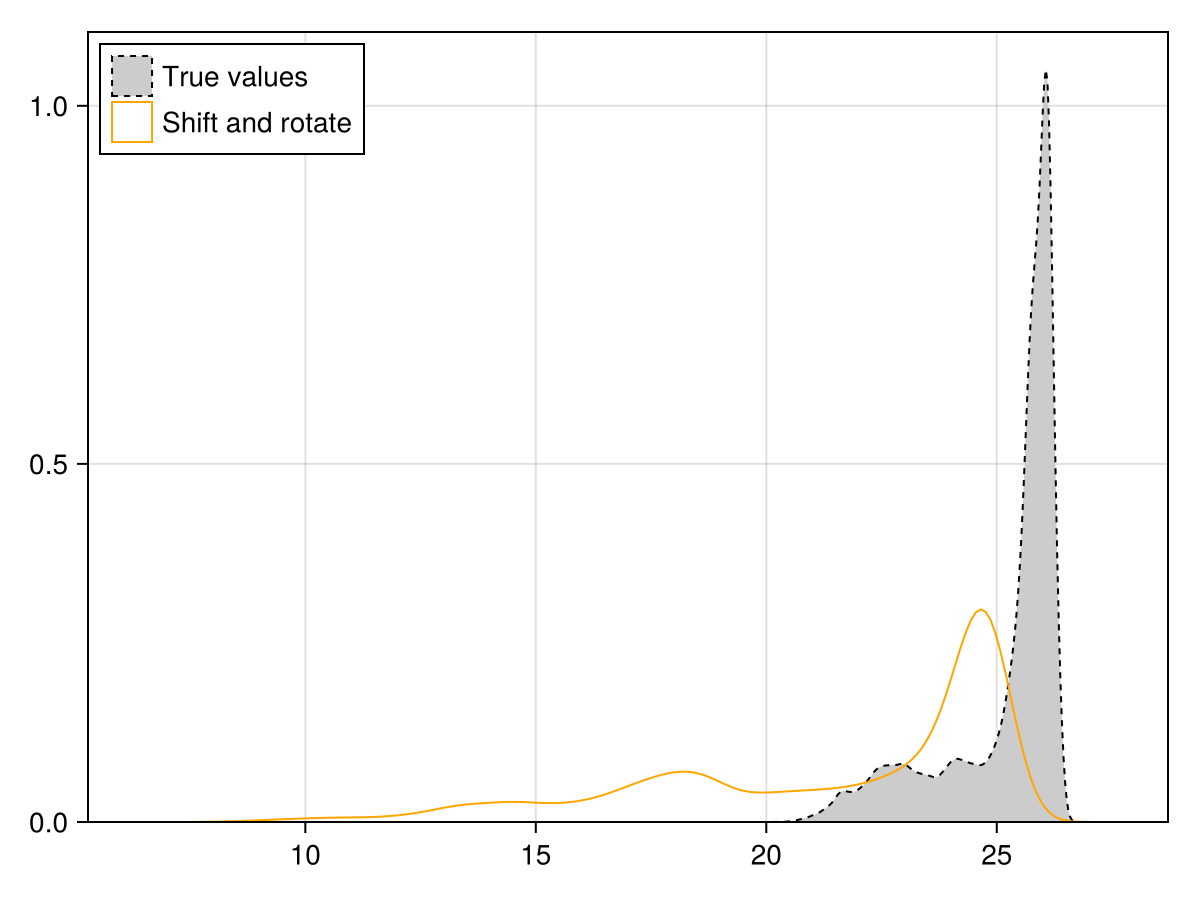
Colorbar(f[1, 2], hm; label = "Average temperature")Dealing with different values distributions
compare the distributions
Code for the figure
f = Figure()
ax = Axis(f[1, 1])
density!(
    ax,
    X[1];
    label = "True values",
    color = :grey80,
    strokecolor = :black,
    linestyle = :dash,
    strokewidth = 1,
)
density!(
    ax,
    M[1];
    label = "Shift and rotate",
    color = :transparent,
    strokecolor = :orange,
    linestyle = :solid,
    strokewidth = 1,
)
axislegend(ax; position = :lt)
ylims!(ax; low = 0)
Now, also ensure that although the spatial structure of this layer has changed, it should have the same distribution of values as the original layer. This can be done with the quantile transfer function:
Q = quantiletransfer(M, X);This function will first calculate the quantiles of every cell in the first (target) layer, then replace by the value corresponding to this quantile in the second (reference) layer. As a result, the distribution of the target layer is updated to become that of the reference layer.
Uses of quantile transfer
This can be used to ask all sorts of very fun questions, like "Where would reindeer live in Malawi if it had the same climate as Norway?". But more importantly, in the context of shift and rotate, this allows us to change the spatial structure of the predictors while keeping their range and distribution identical. Note that this may not keep the joint distribution, and this can be measured as in the covariate shift.
We check that the updated layer has the correct distribution, which is to say, the same as the original layer.
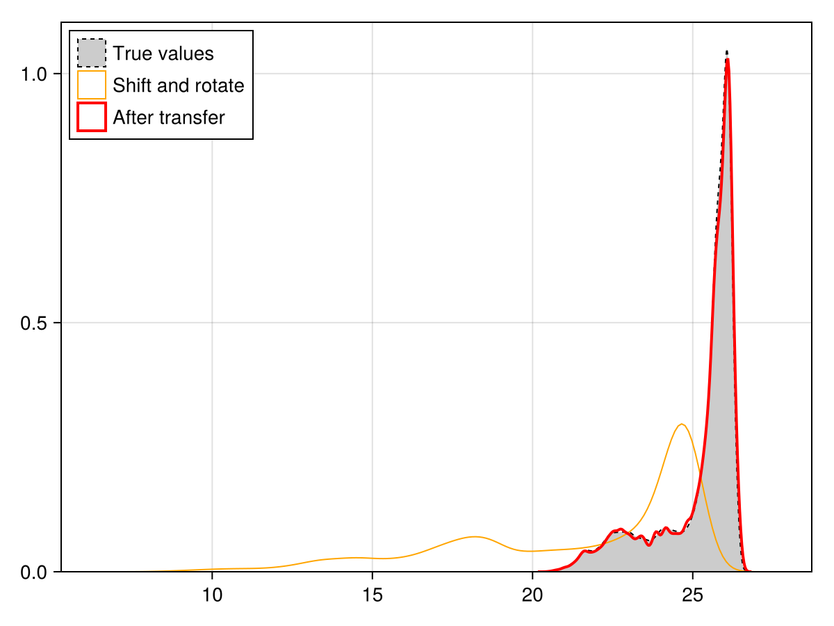
Code for the figure
f = Figure()
ax = Axis(f[1, 1])
density!(
    ax,
    X[1];
    label = "True values",
    color = :grey80,
    strokecolor = :black,
    linestyle = :dash,
    strokewidth = 1,
)
density!(
    ax,
    M[1];
    label = "Shift and rotate",
    color = :transparent,
    strokecolor = :orange,
    linestyle = :solid,
    strokewidth = 1,
)
density!(
    ax,
    Q[1];
    label = "After transfer",
    color = :transparent,
    strokecolor = :red,
    strokewidth = 2,
)
axislegend(ax; position = :lt)
ylims!(ax; low = 0)
Now that we have generated our null sample, we can move on to comparing the performance of SDMs.
Comparing model performance
We generate a series of pseudo-absences. Note that which layer we do it on is not really important, because all three (original, shift and rotate, quantile transfer) have the same coverage.
presencelayer = mask(X[1], records)
background = pseudoabsencemask(BetweenRadius, presencelayer; closer = 10.0, further = 40.0)
absencelayer = backgroundpoints(background, 2sum(presencelayer))
🗺️ A 313 × 174 layer with 27268 Bool cells
Spatial Reference System: +proj=longlat +datum=WGS84 +no_defsWe start by training the "true" model, on observed data and layers:
model = SDM(RawData, NaiveBayes, X, presencelayer, absencelayer)
variables!(model, ForwardSelection)
☑️ RawData → NaiveBayes → P(x) ≥ 0.478 🗺️The next model we train is on the shifted layers (but without quantile transfer, meaning that they carry their data distribution from the location they were sampled from):
null = SDM(RawData, NaiveBayes, M, presencelayer, absencelayer)
variables!(null, ForwardSelection)
☑️ RawData → NaiveBayes → P(x) ≥ 0.481 🗺️Finally, we train the model on the shifted data but with the corrected distribution:
cnull = SDM(RawData, NaiveBayes, Q, presencelayer, absencelayer)
variables!(cnull, ForwardSelection)
☑️ RawData → NaiveBayes → P(x) ≥ 0.624 🗺️Variable selection and model performance
Note that we are selecting the variables independently for each model here, which is different than comparing the performance of a model including the selected variables, against randomly shifted predictors. The choice of the null sample must, as always, match the null hypothesis.
We can now proceed to cross-validate these models (using the same folds, so that the performances are directly comparable):
folds = kfold(model)
cvm = crossvalidate(model, folds);
cvn = crossvalidate(null, folds);
cvc = crossvalidate(cnull, folds);
And we massage these data into a table, to print it:
ms = [mcc, ppv, npv, f1]
CVM = permutedims([
    m(c) for m in ms, c in [
        cvm.training,
        cvm.validation,
        cvn.training,
        cvn.validation,
        cvc.training,
        cvc.validation,
    ]
]);
CVM = hcat(
    ["Real data", "", "Shift & rotate", "", "Quant. transf.", ""],
    ["Train.", "Val.", "Train.", "Val.", "Train.", "Val."],
    CVM,
);
These are the results:
pretty_table(
    CVM;
    alignment = [:l, :l, :c, :c, :c, :c],
    backend = :markdown,
    column_labels = [""; "Dataset"; string.(ms)],
    formatters = [fmt__printf("%5.3f", [3, 4, 5, 6])],
)| Dataset | mcc | ppv | npv | f1 | |
|---|---|---|---|---|---|
| Real data | Train. | 0.842 | 0.844 | 0.976 | 0.897 |
| Val. | 0.843 | 0.846 | 0.977 | 0.898 | |
| Shift & rotate | Train. | 0.920 | 0.952 | 0.970 | 0.947 |
| Val. | 0.921 | 0.955 | 0.969 | 0.947 | |
| Quant. transf. | Train. | 0.901 | 0.930 | 0.968 | 0.935 |
| Val. | 0.901 | 0.932 | 0.968 | 0.935 |
By repeating this process multiple time, we can get a distribution of the expected performance after the layers have been shifted. Finally, we can map the different predictions, that show what the prediction of the species range would be based on the three datasets.
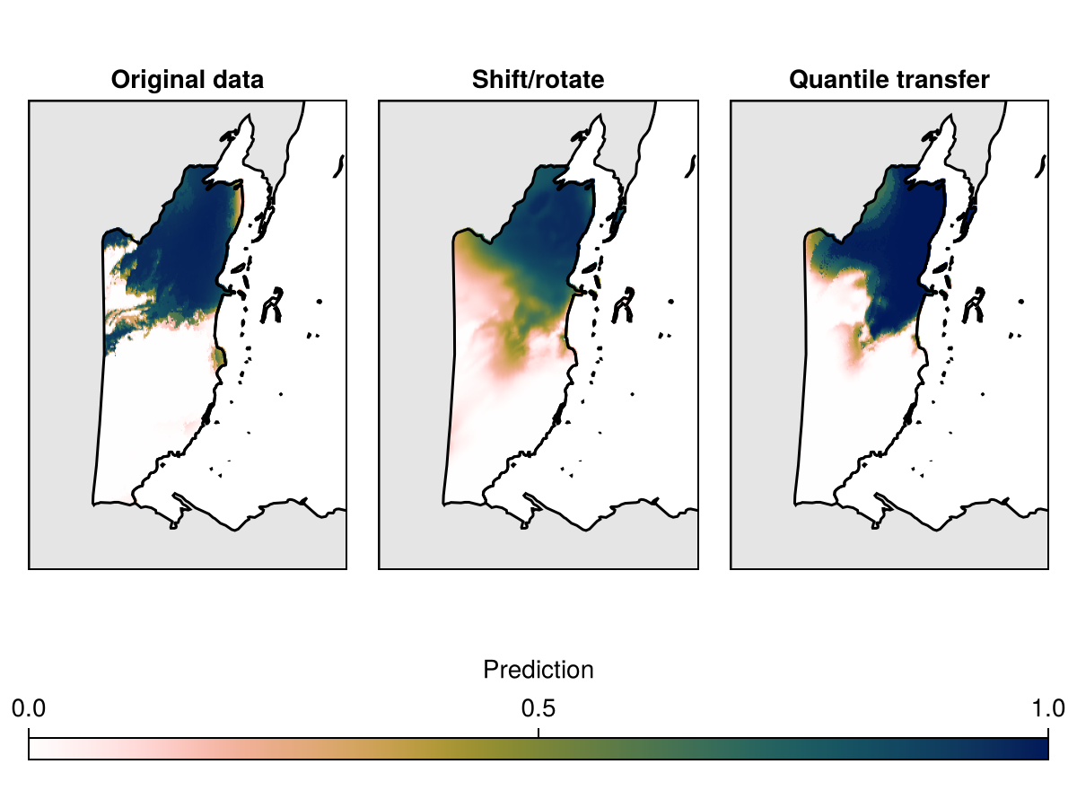
Code for the figure
f = Figure()
axs = [
    Axis(f[1, 1]; aspect = DataAspect(), title = "Original data"),
    Axis(f[1, 2]; aspect = DataAspect(), title = "Shift/rotate"),
    Axis(f[1, 3]; aspect = DataAspect(), title = "Quantile transfer"),
]
for i in 1:3
    poly!(axs[i], clip(landmass, SDT.boundingbox(X[1]; padding = 0.5)); color = :grey90)
end
hm = heatmap!(
    axs[1],
    predict(model, X; threshold = false);
    colorrange = (0, 1),
    colormap = Reverse(:batlowW),
)
heatmap!(
    axs[2],
    predict(null, M; threshold = false);
    colorrange = (0, 1),
    colormap = Reverse(:batlowW),
)
heatmap!(
    axs[3],
    predict(cnull, Q; threshold = false);
    colorrange = (0, 1),
    colormap = Reverse(:batlowW),
)
for i in 1:3
    lines!(axs[i], clip(landmass, SDT.boundingbox(X[1]; padding = 0.5)); color = :black)
    lines!(axs[i], aoi; color = :black)
    hidedecorations!(axs[i])
end
Colorbar(
    f[2, 1:3],
    hm;
    label = "Prediction",
    tellheight = false,
    tellwidth = false,
    vertical = false,
)
rowsize!(f.layout, 2, Relative(0.1))
Related documentation
SimpleSDMLayers.shiftandrotate Function
shiftandrotate(L::SDMLayer, P::SDMLayer, rotator)Returns the output of shifting and rotating the layer L on the layer P, according to a rotator function, obtained with for example findrotation. This function generates a copy of L.
SimpleSDMLayers.findrotation Function
findrotation(L, P; rotations=(-180., 180), maxiter=50)Find a possible rotation for the shiftandrotate function, by attempting to move a target layer L until all of the shifted and rotated coordinates are valid coordinates in the layer P. The range of angles to explore is given as keywords, and the function accepts a maxiter argument after which, if no rotation is found, it returns nothing.
The output of this method is either nothing (no valid rotation found), or a rotator function (see the documentation for rotator).
Note that it is almost always a valid strategy to look for shifts and rotations on a raster at a coarser resolution.
sourceSimpleSDMLayers.quantiletransfer Function
quantiletransfer(target, reference)Non-mutating version of quantiletransfer!
SimpleSDMLayers.quantiletransfer! Function
quantiletransfer!(target::SDMLayer{T}, reference::SDMLayer) where {T <: Real}Replaces the values in the target layer so that they follow the distribution of the values in the reference layer. This works by (i) identifying the quantile of each cell in the target layer, then (ii) replacing this with the value for the same quantile in the reference layer.
References
- Ridder, G. I.; Hardy, O. J. and Ovaskainen, O. (2024). Generating spatially realistic environmental null models with the shift‐&‐rotate approach helps evaluate false positives in species distribution modelling. Methods in Ecology and Evolution. Publisher: Wiley.