Integration with SpatialBoundaries
In this tutorial, we will use methods from SpatialBoundaries (Strydom and Poisot, 2023) to estimate boundaries for the presence of the trees in the landscape.
using SpeciesDistributionToolkit
using StatsBase
using Statistics
using CairoMakie
The SpatialBoundaries package works with SpeciesDistributionToolkit through an extension, so that you can get access to the integration when SpatialBoundaries is loaded in your project:
using SpatialBoundaries Because there are four different layers in the EarthEnv database that represent different types of woody cover, we will use the overall mean wombling across all classes of landscape that correspond to trees.
First, we get a region of interest, as well as the relevant landcover categories.
borders = getpolygon(PolygonData(NaturalEarth, Countries))
region = borders["Austria"]
bbox = SpeciesDistributionToolkit.boundingbox(region; padding=0.3)
borders = clip(borders, bbox)
dataprovider = RasterData(EarthEnv, LandCover)
landcover_classes = layers(dataprovider)
12-element Vector{String}:
"Evergreen/Deciduous Needleleaf Trees"
"Evergreen Broadleaf Trees"
"Deciduous Broadleaf Trees"
"Mixed/Other Trees"
"Shrubs"
"Herbaceous Vegetation"
"Cultivated and Managed Vegetation"
"Regularly Flooded Vegetation"
"Urban/Built-up"
"Snow/Ice"
"Barren"
"Open Water"We need to figure out which of the layers are relevant, which is simply "the layers with trees in their name":
classes_with_trees = findall(contains.(landcover_classes, "Trees"))
landcover = [
    SDMLayer(dataprovider; layer = class, full = true, bbox...)
    for class in classes_with_trees
]
mask!(landcover, region)
4-element Vector{SDMLayer{UInt8}}:
🗺️ A 389 × 988 layer (144630 UInt8 cells)
🗺️ A 389 × 988 layer (144630 UInt8 cells)
🗺️ A 389 × 988 layer (144630 UInt8 cells)
🗺️ A 389 × 988 layer (144630 UInt8 cells)As layers one through four of the EarthEnv data are concerned with data on woody cover (i.e. "Evergreen/Deciduous Needleleaf Trees", "Evergreen Broadleaf Trees", "Deciduous Broadleaf Trees", and "Mixed/Other Trees") we will work with only these layers. For a quick idea we of what the raw landcover data looks like we can sum these four layers and plot the total woody cover:
trees = reduce(+, landcover)🗺️ A 389 × 988 layer with 144630 UInt8 cells
Spatial Reference System: +proj=longlat +datum=WGS84 +no_defsLet's check that the layer looks correct:
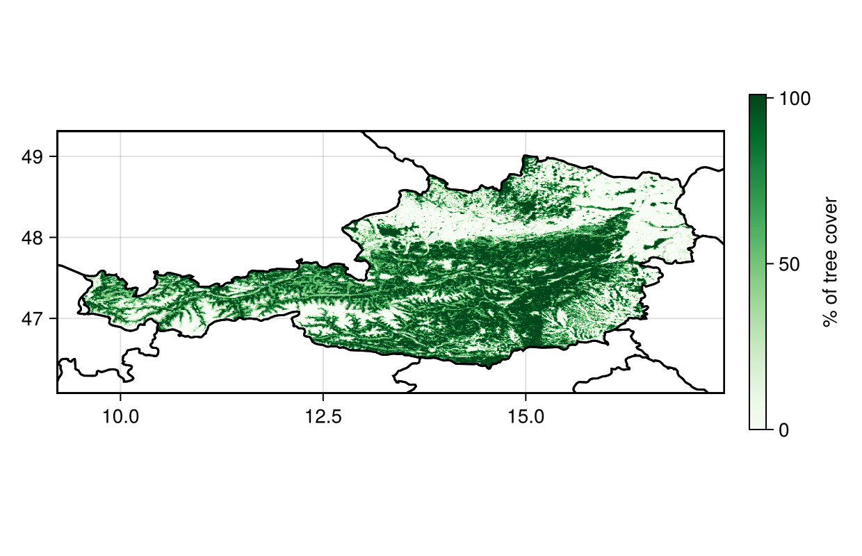
Code for the figure
f = Figure(; size=(620,400))
ax = Axis(f[1,1], aspect=DataAspect())
hm = heatmap!(ax, trees; colormap = :Greens)
lines!(ax, borders, color=:black)
Colorbar(f[1,2], hm, label="% of tree cover", height=Relative(0.7))
Because there are several layers, we can pass them to the wombling function directly, to return the mean rate and mean angular direction:
W = wombling(landcover);In this case, because we are interested in all the trees, we will work directly on the summed layers:
W = wombling(trees);We start by looking at the rate of change - this is useful to pinpoint which area are likely to be identified as zones of transition. The rate of change is in units of the measurement, which in this case is percentages. Larger values correspond to sharper transitions.
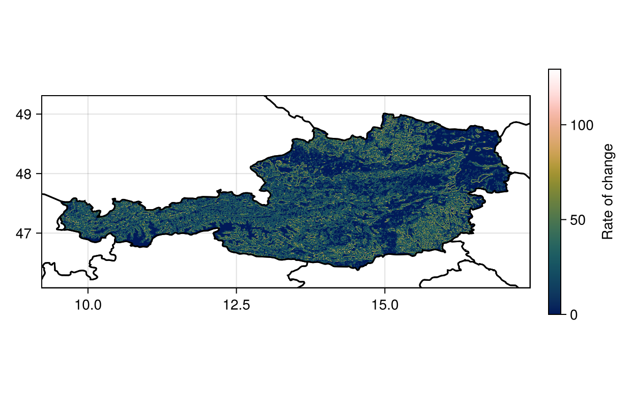
Code for the figure
f = Figure(; size=(620,400))
ax = Axis(f[1,1], aspect=DataAspect())
hm = heatmap!(ax, W.rate, colormap=:batlowW)
lines!(ax, borders, color=:black)
Colorbar(f[1,2], hm, label="Rate of change", height=Relative(0.7))
We can get a sense of which cells are candidate boundaries, by picking the top 15%:
cutoff = quantile(W.rate, 0.85)
candidates = (W.rate .>= cutoff)
🗺️ A 388 × 987 layer with 142864 Bool cells
Spatial Reference System: +proj=longlat +datum=WGS84 +no_defsWe can plot these candidate points identified this way - these correspond to potential boundaries between low and high value area:
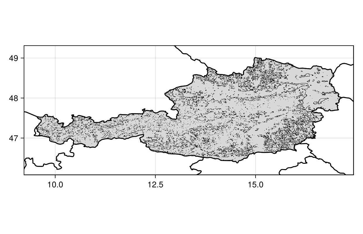
Code for the figure
f = Figure(; size=(620,400))
ax = Axis(f[1,1], aspect=DataAspect())
heatmap!(ax, candidates; colormap = [:grey85, :black])
lines!(ax, borders, color=:black)
The wombling function will also return a layer that gives the direction of change. The direction is expressed as wind direction, i.e. the direction in which the change originates.
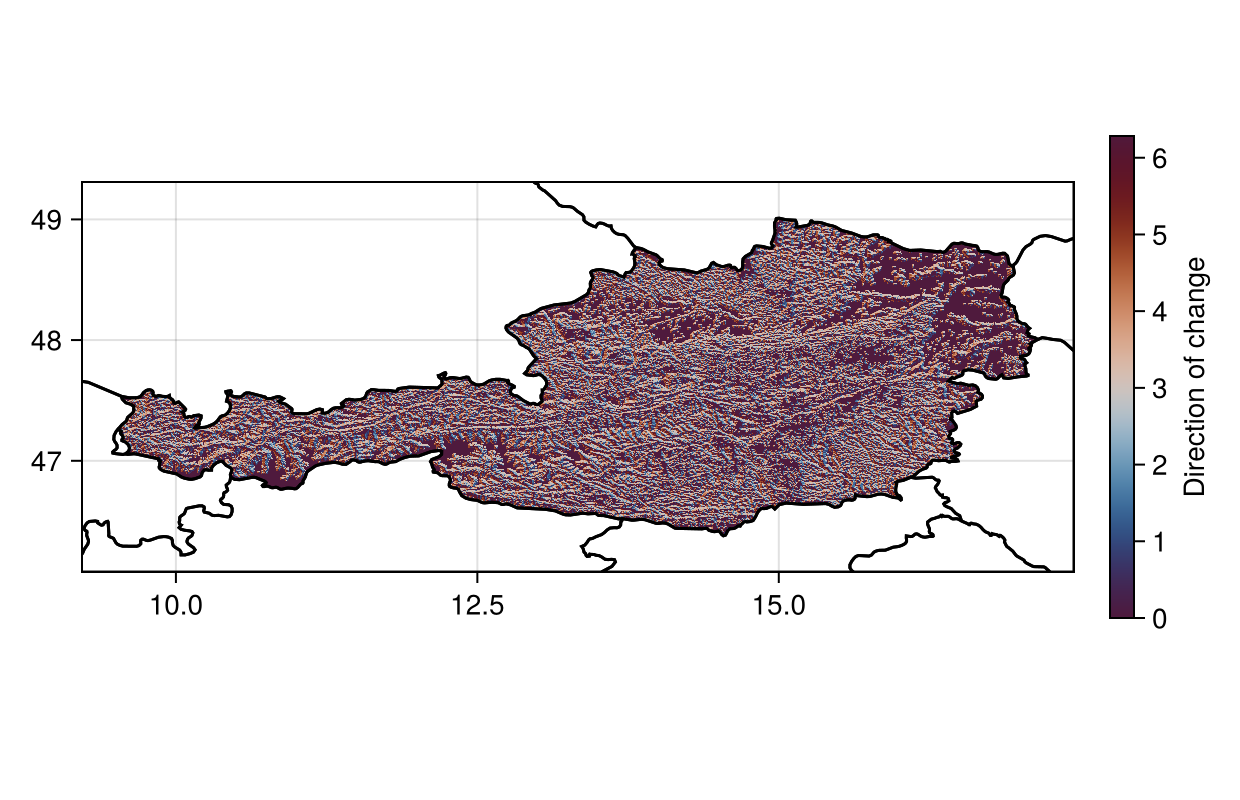
Code for the figure
f = Figure(; size=(620,400))
ax = Axis(f[1,1], aspect=DataAspect())
hm = heatmap!(ax, deg2rad.(W.direction), colormap=:vikO, colorrange=(0, 2π))
lines!(ax, borders, color=:black)
Colorbar(f[1,2], hm, label="Direction of change", height=Relative(0.7))
We can also plot the direction of change as radial plots to get an idea of the prominent direction of change.
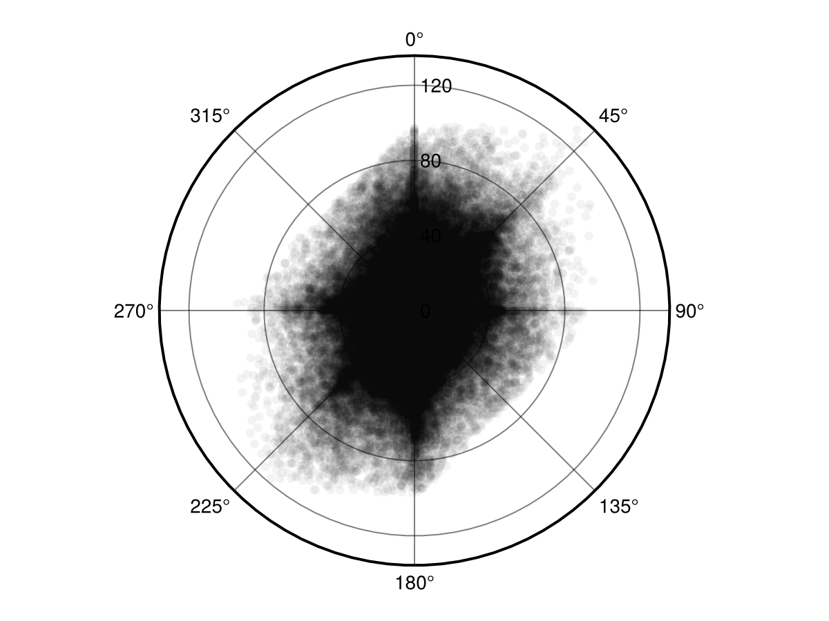
Code for the figure
f = Figure()
ax = PolarAxis(f[1, 1]; theta_0 = -pi / 2, direction = -1)
scatter!(ax, deg2rad.(W.direction), W.rate, alpha=0.05, color=:black)
References
- Strydom, T. and Poisot, T. (2023). SpatialBoundaries.jl: edge detection using spatial wombling. Ecography 2023. Publisher: Wiley.