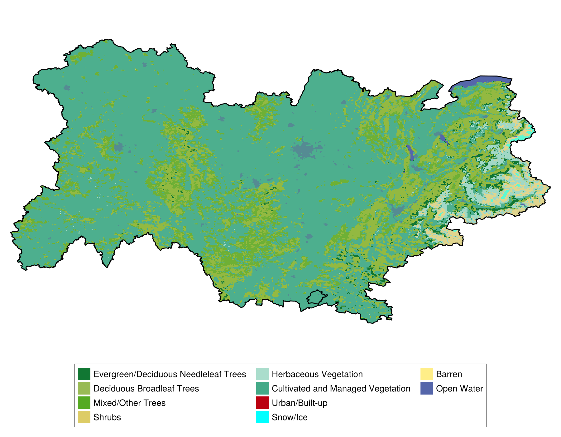
Creating a landcover consensus map

In this vignette, we will look at the different landcover classes in the Alps mountain range. This is an opportunity to see how we can edit, mask, and aggregate data for processing.

using SpeciesDistributionToolkit
using CairoMakie

POL = SpeciesDistributionToolkit.openstreetmap("Alps")
spatial_extent = SpeciesDistributionToolkit.boundingbox(POL)

(left = 5.045573711395264, right = 16.6058349609375, bottom = 43.40773010253906, top = 48.40929412841797)

Defining a bounding box is important because, although we can clip any layer, the package will only read what is required. For large data (like landcover data), this is a significant improvement in memory footprint.

We now define our data provider, composed of a data source (EarthEnv) and a dataset (LandCover).

dataprovider = RasterData(EarthEnv, LandCover)

RasterData{EarthEnv, LandCover}(EarthEnv, LandCover)

It is good practice to check which layers are provided:

landcover_types = layers(dataprovider)

12-element Vector{String}:
 "Evergreen/Deciduous Needleleaf Trees"
 "Evergreen Broadleaf Trees"
 "Deciduous Broadleaf Trees"
 "Mixed/Other Trees"
 "Shrubs"
 "Herbaceous Vegetation"
 "Cultivated and Managed Vegetation"
 "Regularly Flooded Vegetation"
 "Urban/Built-up"
 "Snow/Ice"
 "Barren"
 "Open Water"

For more information, you can also refer to the URL of the original dataset:

SimpleSDMDatasets.url(dataprovider)

"https://www.earthenv.org/landcover"

We can download all the layers using a list comprehension. Note that the name (stack) is a little misleading, as the packages have no concept of what a stack of raster is.

stack = [
    SDMLayer(dataprovider; layer = layer, full = true, spatial_extent...) for
    layer in landcover_types
];

We then mask the layers using the polygon we are interested in:

mask!(stack, POL)

12-element Vector{SDMLayer{UInt8}}:
 🗺️  A 602 × 1388 layer (305963 UInt8 cells)
 🗺️  A 602 × 1388 layer (305963 UInt8 cells)
 🗺️  A 602 × 1388 layer (305963 UInt8 cells)
 🗺️  A 602 × 1388 layer (305963 UInt8 cells)
 🗺️  A 602 × 1388 layer (305963 UInt8 cells)
 🗺️  A 602 × 1388 layer (305963 UInt8 cells)
 🗺️  A 602 × 1388 layer (305963 UInt8 cells)
 🗺️  A 602 × 1388 layer (305963 UInt8 cells)
 🗺️  A 602 × 1388 layer (305963 UInt8 cells)
 🗺️  A 602 × 1388 layer (305963 UInt8 cells)
 🗺️  A 602 × 1388 layer (305963 UInt8 cells)
 🗺️  A 602 × 1388 layer (305963 UInt8 cells)

At this point, we are ready to get the most important land use category for each pixel, using the mosaic function:

consensus = mosaic(argmax, stack)

🗺️  A 602 × 1388 layer with 305963 Int64 cells
   Projection: +proj=longlat +datum=WGS84 +no_defs

In order to represent the output, we will define a color palette corresponding to the different categories in our data:

landcover_colors = [
    colorant"#117733",
    colorant"#668822",
    colorant"#99BB55",
    colorant"#55aa22",
    colorant"#ddcc66",
    colorant"#aaddcc",
    colorant"#44aa88",
    colorant"#88bbaa",
    colorant"#bb0011",
    :aqua,
    colorant"#FFEE88",
    colorant"#5566AA",
];

We can check which categories are actually represented in the consensus map:

repr = sort(unique(values(consensus)))

11-element Vector{Int64}:
  1
  3
  4
  5
  6
  7
  8
  9
 10
 11
 12

We can now create our plot:

Code for the figure

fig = Figure(; size = (900, 700))
panel = Axis(
    fig[1, 1];
    xlabel = "Easting",
    ylabel = "Northing",
    aspect = DataAspect(),
)
hidedecorations!(panel)
hidespines!(panel)
heatmap!(
    panel,
    consensus;
    colormap = landcover_colors[repr],
)
lines!(panel, POL, color=:black)
Legend(
    fig[2, 1],
    [PolyElement(; color = landcover_colors[repr][i]) for i in eachindex(landcover_colors[repr])],
    landcover_types[repr];
    orientation = :horizontal,
    nbanks = 4,
)