Boosting and calibrating a probabilistic classifier
In this vignette, we will see how we can use AdaBoost to turn a mediocre model into a less mediocre one.
using SpeciesDistributionToolkit
const SDT = SpeciesDistributionToolkit
using CairoMakie
We work on the same data as for the previous SDM tutorials:
POL = getpolygon(PolygonData(OpenStreetMap, Places); place = "Switzerland")
presences = GBIF.download("10.15468/dl.wye52h")
provider = RasterData(CHELSA2, BioClim)
L = SDMLayer{Float32}[
    SDMLayer(
        provider;
        layer = x,
        SDT.boundingbox(POL; padding = 0.0)...,
    ) for x in 1:19
];
mask!(L, POL)
19-element Vector{SDMLayer{Float32}}:
🗺️ A 240 × 546 layer (70065 Float32 cells)
🗺️ A 240 × 546 layer (70065 Float32 cells)
🗺️ A 240 × 546 layer (70065 Float32 cells)
🗺️ A 240 × 546 layer (70065 Float32 cells)
🗺️ A 240 × 546 layer (70065 Float32 cells)
🗺️ A 240 × 546 layer (70065 Float32 cells)
🗺️ A 240 × 546 layer (70065 Float32 cells)
🗺️ A 240 × 546 layer (70065 Float32 cells)
🗺️ A 240 × 546 layer (70065 Float32 cells)
🗺️ A 240 × 546 layer (70065 Float32 cells)
🗺️ A 240 × 546 layer (70065 Float32 cells)
🗺️ A 240 × 546 layer (70065 Float32 cells)
🗺️ A 240 × 546 layer (70065 Float32 cells)
🗺️ A 240 × 546 layer (70065 Float32 cells)
🗺️ A 240 × 546 layer (70065 Float32 cells)
🗺️ A 240 × 546 layer (70065 Float32 cells)
🗺️ A 240 × 546 layer (70065 Float32 cells)
🗺️ A 240 × 546 layer (70065 Float32 cells)
🗺️ A 240 × 546 layer (70065 Float32 cells)We generate some pseudo-absence data:
presencelayer = mask(first(L), presences)
background = pseudoabsencemask(DistanceToEvent, presencelayer)
bgpoints = backgroundpoints(nodata(background, d -> d < 4), 2sum(presencelayer))
🗺️ A 240 × 546 layer with 46351 Bool cells
Projection: +proj=longlat +datum=WGS84 +no_defsThis is the dataset we start from:
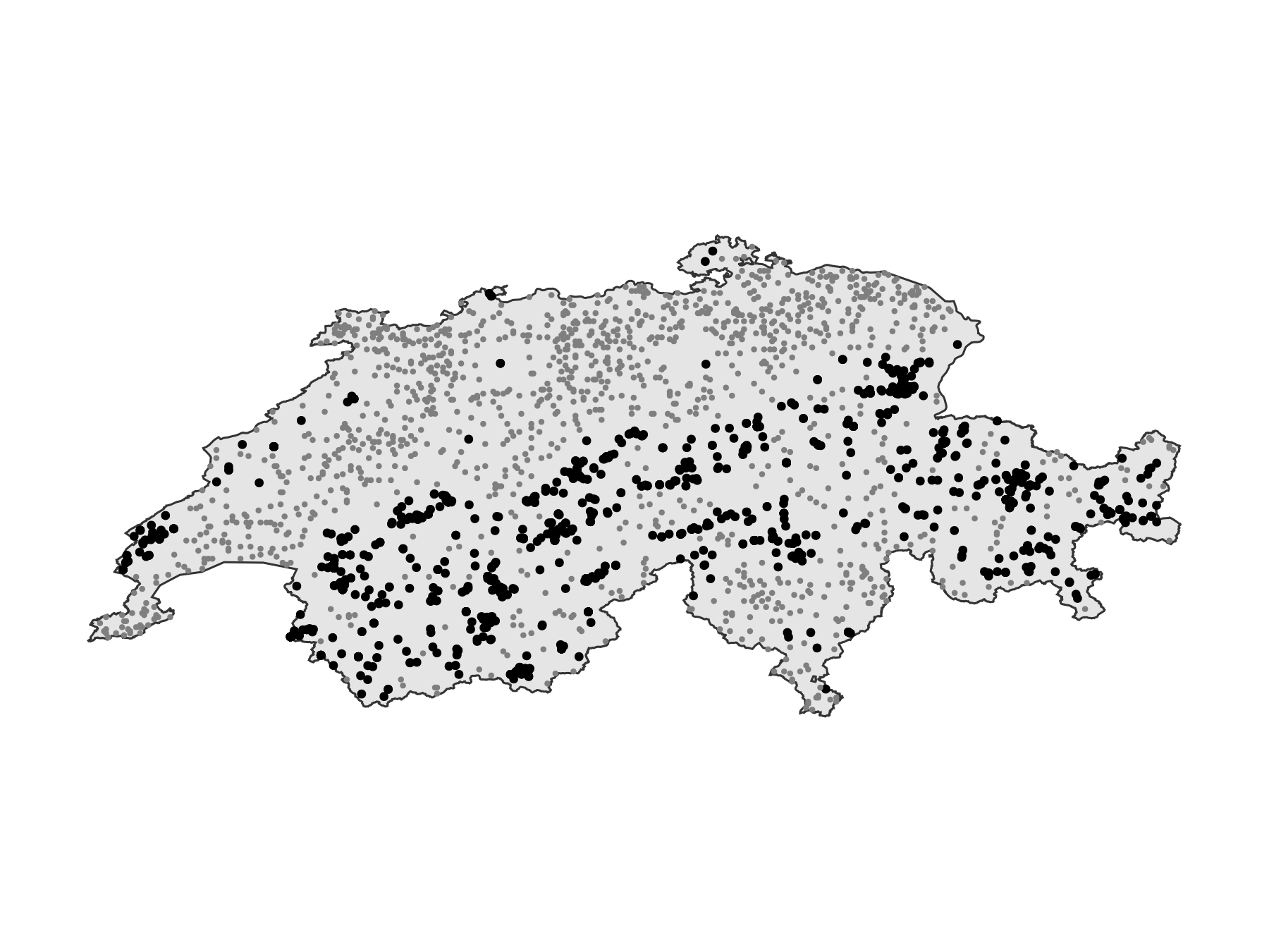
Code for the figure
fig = Figure()
ax = Axis(fig[1, 1]; aspect = DataAspect())
poly!(ax, POL; color = :grey90, strokewidth = 1, strokecolor = :grey20)
scatter!(ax, presences; color = :black, markersize = 6)
scatter!(ax, bgpoints; color = :grey50, markersize = 4)
hidedecorations!(ax)
hidespines!(ax)
Before building the boosting model, we need to construct a weak learner.
The BIOCLIM model (Booth et al., 2014) is one of the first SDM that was ever published. Because it is a climate envelope model (locations within the extrema of environmental variables for observed presences are assumed suitable, more or less), it does not usually give really good predictions. BIOCLIM underfits, and for this reason it is also a good candidate for boosting. Naive Bayes classifiers are similarly suitable for AdaBoost: they tend to achieve a good enough performance in aggregate, but due to the way they learn from the data, they rarely excel at any single prediction.
The traditional lore is that AdaBoost should be used only with really weak classifiers, but Wyner et al. (2017) have convincing arguments in favor of treating it more like a random forest, by showing that it also works with comparatively stronger learners. In keeping with this idea, we will train a moderately deep tree as our base classifier.
sdm = SDM(RawData, DecisionTree, L, presencelayer, bgpoints)
hyperparameters!(classifier(sdm), :maxdepth, 4)
hyperparameters!(classifier(sdm), :maxnodes, 4)
DecisionTree(SDeMo.DecisionNode(nothing, nothing, nothing, 0, 0.0, 0.5, false), 4, 4)This tree is not quite a decision stump (a one-node tree), but they are relatively small, so a single one of them is unlikely to give a good prediction. We can train the model and generate the initial prediction:
train!(sdm)
prd = predict(sdm, L; threshold = false)
🗺️ A 240 × 546 layer with 70065 Float64 cells
Projection: +proj=longlat +datum=WGS84 +no_defsAs expected, although it roughly identifies the range of the species, it is not doing a spectacular job at it. This model is a good candidate for boosting.
Code for the figure
fg, ax, pl = heatmap(prd; colormap = :tempo, colorrange = (0, 1))
ax.aspect = DataAspect()
hidedecorations!(ax)
hidespines!(ax)
lines!(ax, POL; color = :grey20)
Colorbar(fg[1, 2], pl; height = Relative(0.6))
To train this model using the AdaBoost algorithm, we wrap it into an AdaBoost object, and specify the number of iterations (how many learners we want to train). The default is 50.
bst = AdaBoost(sdm; iterations = 60)AdaBoost {RawData → DecisionTree → P(x) ≥ 0.035} × 60 iterationsTraining the model is done in the exact same way as other SDeMo models, with one important exception. AdaBoost uses the predicted class (presence/absence) internally, so we will always train learners to return a thresholded prediction. For this reason, even it the threshold argument is used, it will be ignored during training.
train!(bst)AdaBoost {RawData → DecisionTree → P(x) ≥ 0.035} × 60 iterationsWe can look at the weight (i.e. how much a weak learner is trusted during the final prediction) over time. It should decrease, and more than that, it should ideally decrease fast (exponentially). Some learners may have a negative weight, which means that they are consistently wrong. These are counted by flipping their prediction in the final recommendation.
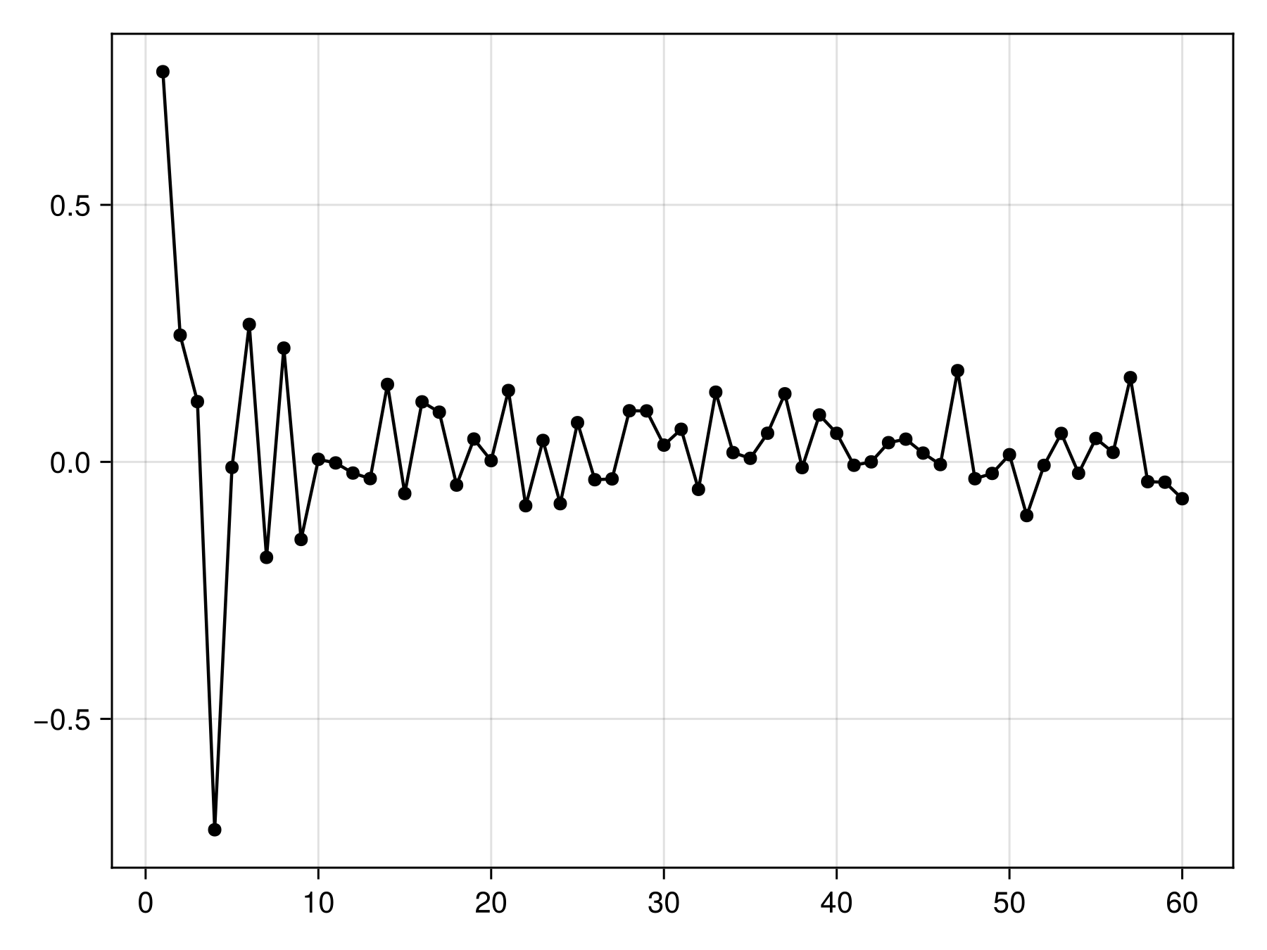
Code for the figure
scatterlines(bst.weights; color = :black)Models with a weight of 0 are not contributing new information to the model. These are expecteed to become increasingly common at later iterations, so it is a good idea to examine the cumulative weights to see whether we get close to a plateau.
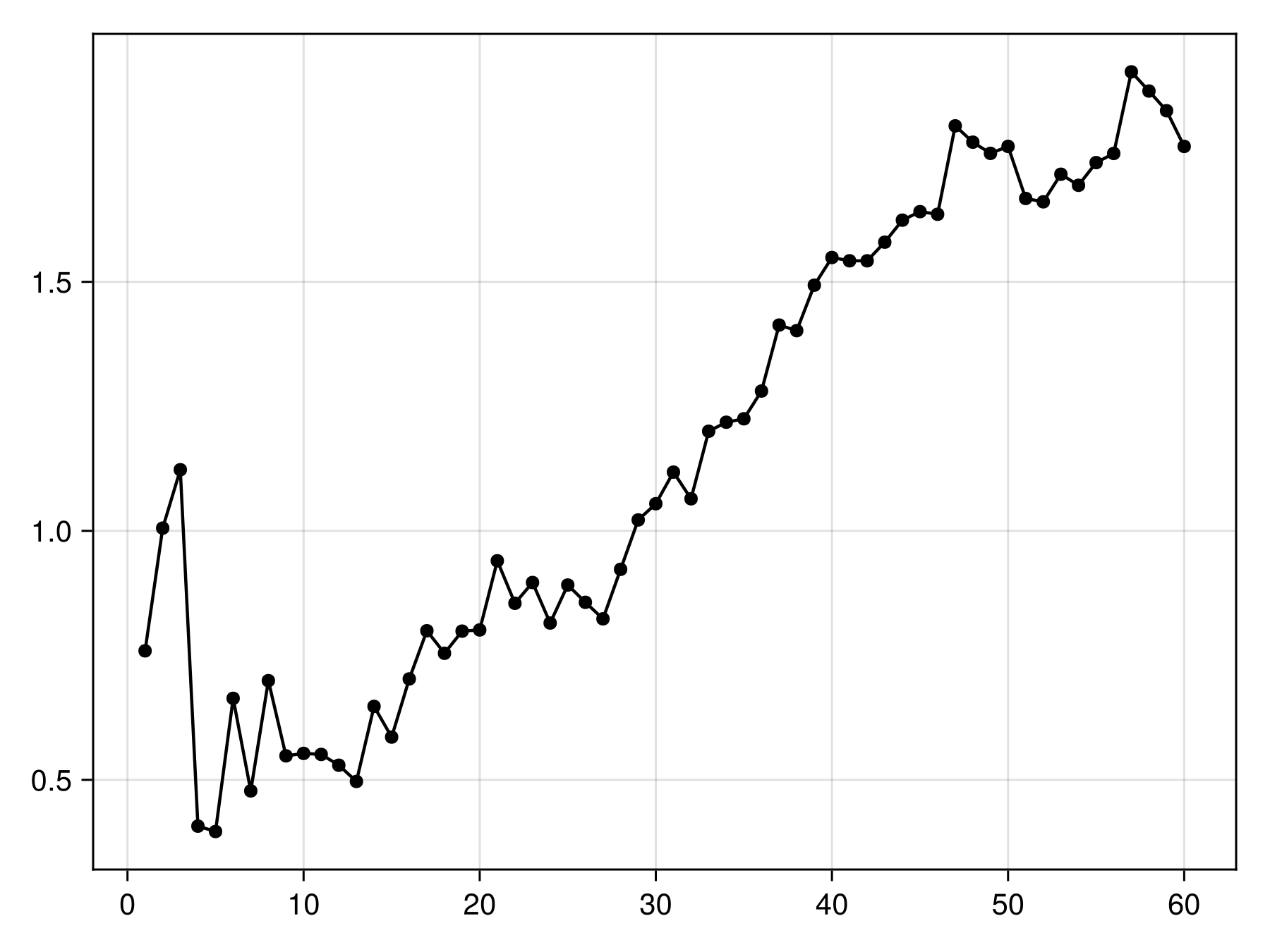
Code for the figure
scatterlines(cumsum(bst.weights); color = :black)This is close enough. We can now apply this model to the bioclimatic variables:
brd = predict(bst, L; threshold = false)🗺️ A 240 × 546 layer with 70065 Float64 cells
Projection: +proj=longlat +datum=WGS84 +no_defsThis gives the following map:
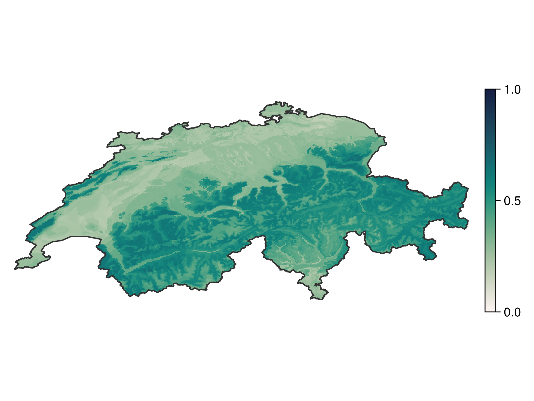
Code for the figure
fg, ax, pl = heatmap(brd; colormap = :tempo, colorrange = (0, 1))
ax.aspect = DataAspect()
hidedecorations!(ax)
hidespines!(ax)
lines!(ax, POL; color = :grey20)
Colorbar(fg[1, 2], pl; height = Relative(0.6))
The scores returned by the boosted model are not calibrated probabilities, so they are centered on 0.5, but have typically low variance. This can be explained by the fact that each component models tends to make one-sided errors near 0 and 1, wich accumulate with more models over time. This problem is typically more serious when adding multiple classifiers together, as with bagging and boosting. Some classifiers tend to exagerate the proportion of extreme values (Naive Bayes classifiers, for example), some others tend to create peaks near values slightly above 0 and below 1 (tree-based methods), while methods like logistic regression typically do a fair job at predicting probabilities.
The type of bias that a classifier accumulates is usually pretty obvious from lookin at the histogram of the results:
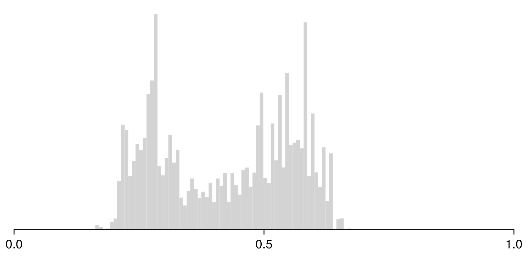
Code for the figure
f = Figure(; size=(600, 300))
ax = Axis(f[1,1]; xlabel="Predicted score")
hist!(ax, brd; color = :lightgrey, bins=70)
hideydecorations!(ax)
hidexdecorations!(ax; ticks = false, ticklabels = false)
hidespines!(ax, :l)
hidespines!(ax, :r)
hidespines!(ax, :t)
xlims!(ax, 0, 1)
tightlimits!(ax)
We can also look at the reliability curve for this model. The reliability curve divides the predictions into bins, and compares the average score on the training data to the proportion of events in the training data. When these two quantities are almost equal, the score outputed by the model is a good prediction of the probability of the event.
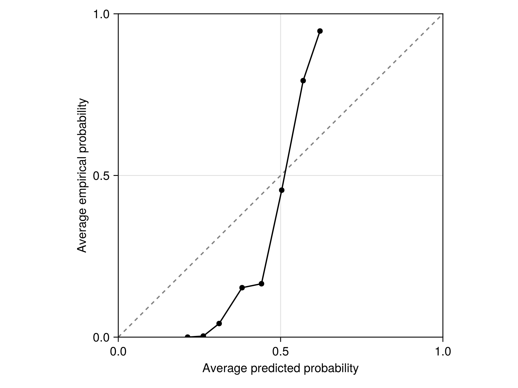
Code for the figure
f = Figure()
ax = Axis(
    f[1, 1];
    aspect = 1,
    xlabel = "Average predicted probability",
    ylabel = "Average empirical probability",
)
lines!(ax, [0, 1], [0, 1]; color = :grey, linestyle = :dash)
xlims!(ax, 0, 1)
ylims!(ax, 0, 1)
scatterlines!(ax, SDeMo.reliability(bst)...; color = :black, label = "Raw scores")
Based on the reliability curve, it is clear that the model outputs are not probabilities. In order to turn these scores into a value that are closer to probabilities, we can estimate calibration parameters for this model:
C = calibrate(bst)SDeMo.PlattCalibration(-29.14362852639919, 14.69823366992224)This step uses the Platt (1999) scaling approach, where the outputs from the model are regressed against the true class probabilities, to attempt to bring the model prediction more in line with true probabilities (Niculescu-Mizil and Caruana, 2005). Internally, the package uses the fast and robust algorithm of Lin et al. (2007).
These parameters can be turned into a correction function:
f = correct(C)#101 (generic function with 1 method)It is a good idea to check that the calibration function is indeed bringing us closer to the 1:1 line, which is to say that it provides us with a score that is closer to a true probability.
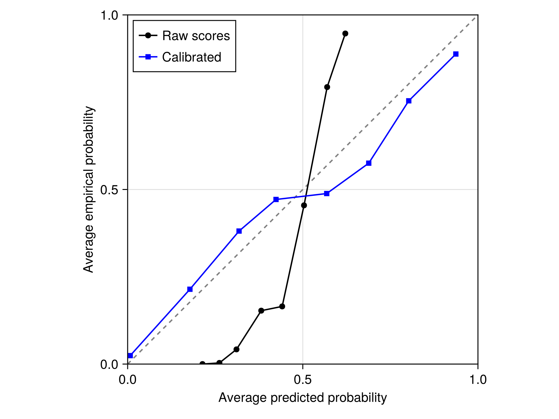
Code for the figure
scatterlines!(
ax,
SDeMo.reliability(bst; link = f)...;
color = :blue,
marker = :rect,
label = "Calibrated",
)
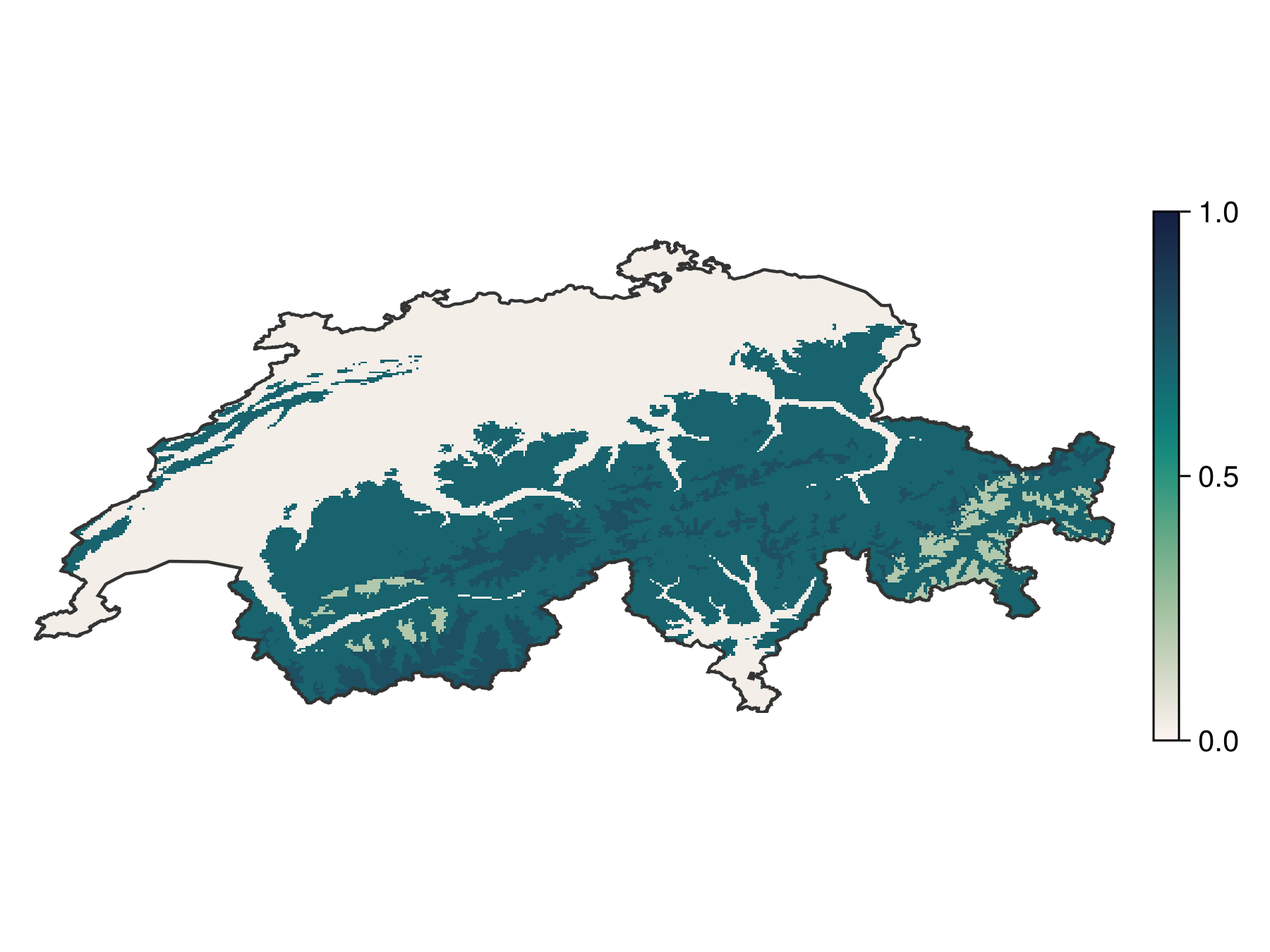
axislegend(ax; position = :lt)Of course the calibration function can be applied to a layer, so we can now use AdaBoost to estimate the probability of species presence. Dormann (2020) has several strong arguments in favor of this approach.
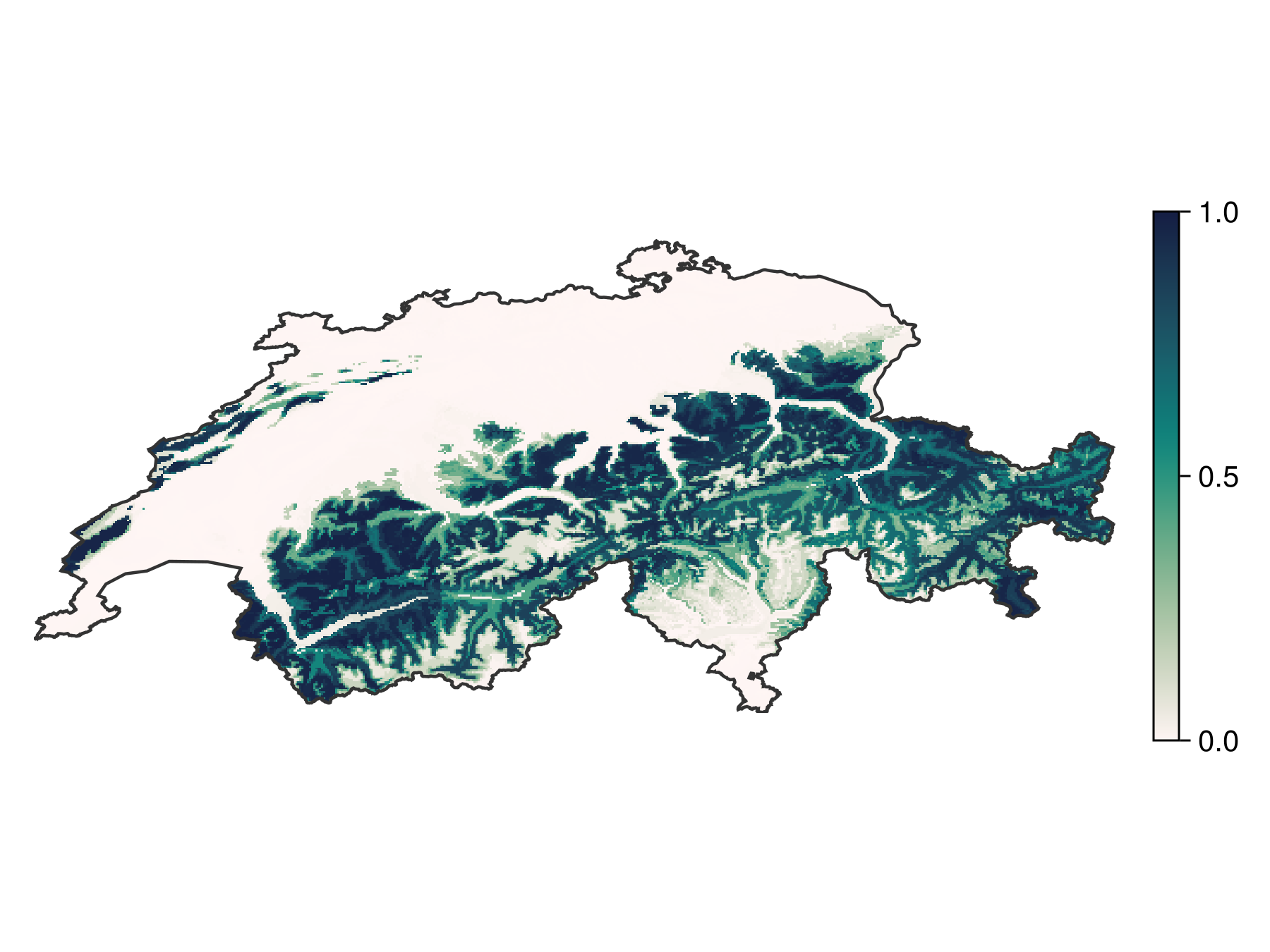
Code for the figure
fg, ax, pl = heatmap(f(brd); colormap = :tempo, colorrange = (0, 1))
ax.aspect = DataAspect()
hidedecorations!(ax)
hidespines!(ax)
lines!(ax, POL; color = :grey20)
Colorbar(fg[1, 2], pl; height = Relative(0.6))
Note that the calibration is not required to obtain a binary map, as the transformation applied to the scores is monotonous. For this reason, the AdaBoost function will internally work on the raw scores, and turn them into binary predictions using thresholding.
The default threshold for AdaBoost is 0.5, which is explained by the fact that the final decision step is a weighted voting based on the sum of all weak learners. We can get the predicted range under both models:
sdm_range = predict(sdm, L)
bst_range = predict(bst, L)
🗺️ A 240 × 546 layer with 70065 Bool cells
Projection: +proj=longlat +datum=WGS84 +no_defsWe now plot the difference, where the areas gained by boosting are in red, and the areas lost by boosting are in light grey. The part of the range that is conserved is in black.
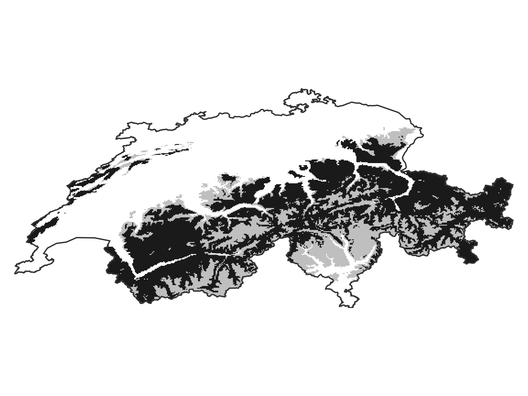
Code for the figure
fg, ax, pl = heatmap(
    gainloss(sdm_range, bst_range);
    colormap = [:firebrick, :grey10, :grey75],
    colorrange = (-1, 1),
)
ax.aspect = DataAspect()
hidedecorations!(ax)
hidespines!(ax)
lines!(ax, POL; color = :grey20)
References
Booth, T. H.; Nix, H. A.; Busby, J. R. and Hutchinson, M. F. (2014), bioclim: the first species distribution modelling package, its early applications and relevance to most current MaxEnt studies. Diversity & distributions 20, 1–9.
Dormann, C. F. (2020). Calibration of probability predictions from machine‐learning and statistical models. Global ecology and biogeography: a journal of macroecology 29, 760–765.
Lin, H.-T.; Lin, C.-J. and Weng, R. C. (2007). A note on Platt’s probabilistic outputs for support vector machines. Machine learning 68, 267–276.
Niculescu-Mizil, A. and Caruana, R. (2005). Obtaining calibrated probabilities from boosting. In: Proceedings of the Twenty-First Conference on Uncertainty in Artificial Intelligence, UAI'05 (AUAI Press); pp. 413–420.
Platt, J. (1999). Probabilistic outputs for support vector machines and comparisons to regularized likelihood methods. In: Advances in large margin classifiers, edited by Smola, A. J.; Bartlett, P.; Schölkopf, B. and Schuurmans, D. (MIT Press).
Wyner, A. J.; Olson, M.; Bleich, J. and Mease, D. (2017). Explaining the success of adaboost and random forests as interpolating classifiers. J. Mach. Learn. Res. 18, 1558–1590.