Integration with SpatialBoundaries

In this tutorial, we will use methods from SpatialBoundaries to estimate boundaries for (i.e. patches of) wooded areas on the Southwestern islands of the Hawaiian Islands using landcover data from the EarthEnv project. The SpatialBoundaries package works with SpeciesDistributionToolkit through an extension, so that you can get access to the integration when SpatialBoundaries is loaded in your project:

using SpeciesDistributionToolkit
using SpatialBoundaries 
using CairoMakie
using StatsBase
using Statistics

Because there are four different layers in the EarthEnv database that represent different types of woody cover, we will use the overall mean wombling value.

First we can start by defining the extent of the Southwestern islands of Hawaii, which can be used to restrict the extraction of the various landcover layers from the EarthEnv database.

hawaii = (left = -160.2, right = -154.5, bottom = 18.6, top = 22.5)
dataprovider = RasterData(EarthEnv, LandCover)
landcover_classes = layers(dataprovider)
landcover = [SDMLayer(dataprovider; layer=class, full=true, hawaii...) for class in landcover_classes]

12-element Vector{SDMLayer{UInt8}}:
 🗺️  A 468 × 684 layer (320112 UInt8 cells)
 🗺️  A 468 × 684 layer (320112 UInt8 cells)
 🗺️  A 468 × 684 layer (320112 UInt8 cells)
 🗺️  A 468 × 684 layer (320112 UInt8 cells)
 🗺️  A 468 × 684 layer (320112 UInt8 cells)
 🗺️  A 468 × 684 layer (320112 UInt8 cells)
 🗺️  A 468 × 684 layer (320112 UInt8 cells)
 🗺️  A 468 × 684 layer (320112 UInt8 cells)
 🗺️  A 468 × 684 layer (320112 UInt8 cells)
 🗺️  A 468 × 684 layer (320112 UInt8 cells)
 🗺️  A 468 × 684 layer (320112 UInt8 cells)
 🗺️  A 468 × 684 layer (320112 UInt8 cells)

We can remove all the areas that contain 100% water from the landcover data as our question of interest is restricted to the terrestrial realm. We do this by using the "Open Water" layer to mask over each of the landcover layers individually:

ow_index = findfirst(isequal("Open Water"), landcover_classes)
not_water = landcover[ow_index] .!== 0x64
nodata!(not_water, false)
[mask!(layer, not_water) for layer in landcover]

12-element Vector{SDMLayer{UInt8}}:
 🗺️  A 468 × 684 layer (21764 UInt8 cells)
 🗺️  A 468 × 684 layer (21764 UInt8 cells)
 🗺️  A 468 × 684 layer (21764 UInt8 cells)
 🗺️  A 468 × 684 layer (21764 UInt8 cells)
 🗺️  A 468 × 684 layer (21764 UInt8 cells)
 🗺️  A 468 × 684 layer (21764 UInt8 cells)
 🗺️  A 468 × 684 layer (21764 UInt8 cells)
 🗺️  A 468 × 684 layer (21764 UInt8 cells)
 🗺️  A 468 × 684 layer (21764 UInt8 cells)
 🗺️  A 468 × 684 layer (21764 UInt8 cells)
 🗺️  A 468 × 684 layer (21764 UInt8 cells)
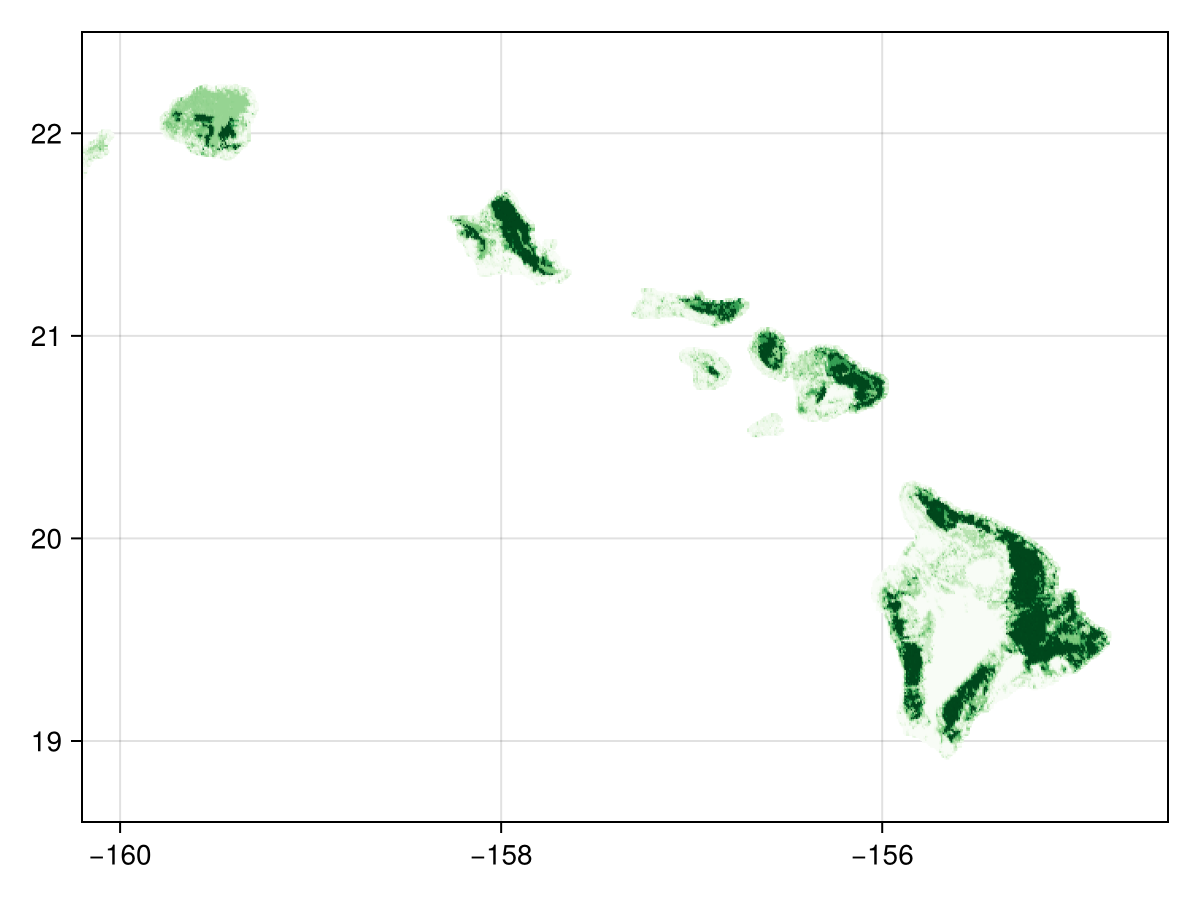
 🗺️  A 468 × 684 layer (21764 UInt8 cells)

As layers one through four of the EarthEnv data are concerned with data on woody cover (i.e. "Evergreen/Deciduous Needleleaf Trees", "Evergreen Broadleaf Trees", "Deciduous Broadleaf Trees", and "Mixed/Other Trees") we will work with only these layers. For a quick idea we of what the raw landcover data looks like we can sum these four layers and plot the total woody cover:

classes_with_trees = findall(contains.(landcover_classes, "Trees"))
tree_lc = convert(SDMLayer{Float64}, reduce(+, landcover[classes_with_trees]))

🗺️  A 468 × 684 layer with 21764 Float64 cells
   Projection: +proj=longlat +datum=WGS84 +no_defs

Let's check that the layer looks correct:

Code for the figure

heatmap(tree_lc; colormap=:Greens)

Because there are several layers, we can pass them to the wombling function directly, to return the mean rate and mean angular direction:

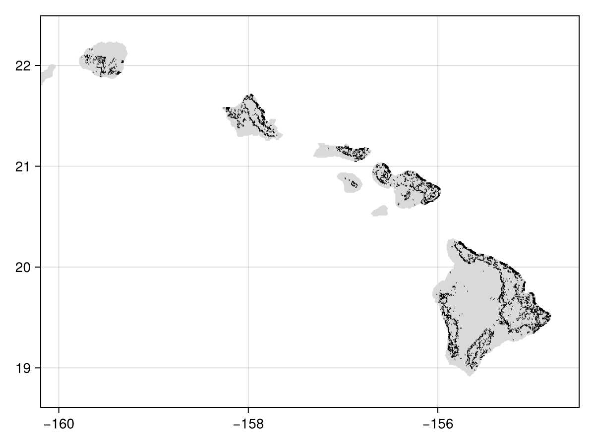
W = wombling(landcover[classes_with_trees]);

We can get a sense of which cells are candidate boundaries, by picking the top 15%:

cutoff = quantile(W.rate, 0.85)
candidates = (W.rate.>=cutoff)

🗺️  A 467 × 683 layer with 20759 Bool cells
   Projection: +proj=longlat +datum=WGS84 +no_defs

We can plot these candidate points identified this way - these correspond to potential boundaries between low and high value area:

Code for the figure

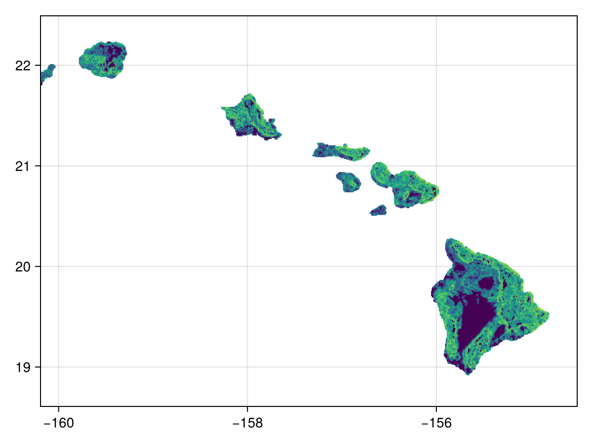
heatmap(candidates, colormap=[:grey85, :black])

We can also look at the (log of the) rate of change - this is useful to pinpoint which area are likely to be identified as zones of transition:

Code for the figure

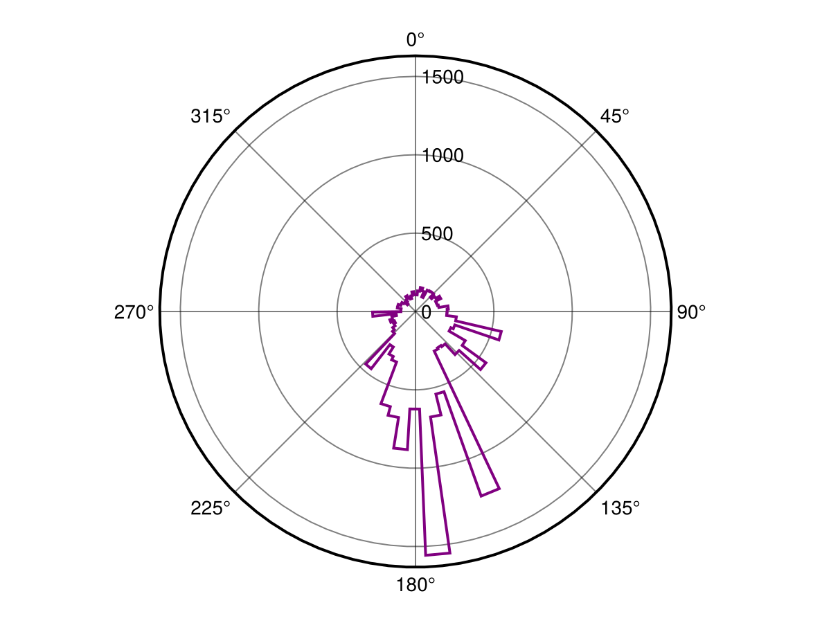
heatmap(log1p.(W.rate))

For this example we will plot the direction of change as radial plots to get an idea of the prominent direction of change. Here we will plot all the direction values from direction for which the rate of change is greater than zero (so as to avoid denoting directions for a slope that does not exist):

direction = mask(W.direction, nodata(W.rate, 0.0))

🗺️  A 467 × 683 layer with 17334 Float64 cells
   Projection: +proj=longlat +datum=WGS84 +no_defs

Because stephist() requires a vector of radians for plotting we must first collect the cells and convert them from degrees to radians. Then we can start by plotting the direction of change of all cells.

Code for the figure

f = Figure()
ax = PolarAxis(f[1, 1], theta_0 = -pi/2, direction = -1)
h = fit(Histogram, deg2rad.(values(direction)); nbins = 100)
stairs!(ax, h.edges[1], h.weights[[axes(h.weights, 1)..., 1]]; color = :purple, linewidth = 2)

References

- Strydom, T. and Poisot, T. (2023). SpatialBoundaries.jl: edge detection using spatial wombling. Ecography 2023.