Conformal prediction of species range
This tutorial goes through some of the steps outlined in Poisot (Dec 2025). We will use conformal prediction to identify areas in space in which a SDM is uncertain about the outcome of presence and absence of the species.
using SpeciesDistributionToolkit
using CairoMakie
We will work on the distribution of Sasquatch observations in Oregon.
records = OccurrencesInterface.__demodata()
landmass = getpolygon(PolygonData(OpenStreetMap, Places); place = "Oregon")
records = Occurrences(mask(records, landmass))
spatial_extent = SpeciesDistributionToolkit.boundingbox(landmass)
(left = -124.70354461669922, right = -116.46315002441406, bottom = 41.99179458618164, top = 46.292396545410156)We will train the model will all 19 BioClim variables from CHELSA2:
provider = RasterData(CHELSA2, BioClim)
L = SDMLayer{Float32}[
    SDMLayer(
        provider;
        layer = x,
        spatial_extent...,
    ) for x in eachindex(layers(provider))
];

mask!(L, landmass)
19-element Vector{SDMLayer{Float32}}:
🗺️ A 517 × 990 layer (411406 Float32 cells)
🗺️ A 517 × 990 layer (411406 Float32 cells)
🗺️ A 517 × 990 layer (411406 Float32 cells)
🗺️ A 517 × 990 layer (411406 Float32 cells)
🗺️ A 517 × 990 layer (411406 Float32 cells)
🗺️ A 517 × 990 layer (411406 Float32 cells)
🗺️ A 517 × 990 layer (411406 Float32 cells)
🗺️ A 517 × 990 layer (411406 Float32 cells)
🗺️ A 517 × 990 layer (411406 Float32 cells)
🗺️ A 517 × 990 layer (411406 Float32 cells)
🗺️ A 517 × 990 layer (411406 Float32 cells)
🗺️ A 517 × 990 layer (411406 Float32 cells)
🗺️ A 517 × 990 layer (411406 Float32 cells)
🗺️ A 517 × 990 layer (411406 Float32 cells)
🗺️ A 517 × 990 layer (411406 Float32 cells)
🗺️ A 517 × 990 layer (411406 Float32 cells)
🗺️ A 517 × 990 layer (411406 Float32 cells)
🗺️ A 517 × 990 layer (411406 Float32 cells)
🗺️ A 517 × 990 layer (411406 Float32 cells)We will generate pseudo-absences at random in a radius around each known observations. The distance between an observation and a pseudo-absence is between 40 and 130 km.
presencelayer = mask(first(L), records)
absencemask =
    pseudoabsencemask(BetweenRadius, presencelayer; closer = 40.0, further = 120.0)
absencelayer = backgroundpoints(absencemask, 2sum(presencelayer))
🗺️ A 517 × 990 layer with 411406 Bool cells
Spatial Reference System: +proj=longlat +datum=WGS84 +no_defsTraining the initial model
The model for this tutorial is a logistic regression, with self-interactions between variables, but no other interactive effects:
model = SDM(RawData, Logistic, L, presencelayer, absencelayer)
hyperparameters!(classifier(model), :interactions, :self)
variables!(model, BackwardSelection)
variables!(model, ForwardSelection)
☑️ RawData → Logistic → P(x) ≥ 0.263 🗺️We start by checking that this model is georeferenced. This is something we will rely on when putting the observations on the map near the end of the tutorial.
isgeoreferenced(model)trueModel performance
Conformal prediction requires a good model - it is important to cross-validate the model before calibrating the conformal predictor.
cv = crossvalidate(model, kfold(model))
println("""
Validation MCC: $(mcc(cv.validation)) ± $(ci(cv.validation))
Training MCC:   $(mcc(cv.training)) ± $(ci(cv.training))
""")
Validation MCC: 0.7889375587966321 ± 0.07548321810685577
Training MCC: 0.7970883478647804 ± 0.0074576168403487075With a trained model, we can make our first (spatial) prediction
Y = predict(model, L; threshold = false)🗺️ A 517 × 990 layer with 411406 Float64 cells
Spatial Reference System: +proj=longlat +datum=WGS84 +no_defs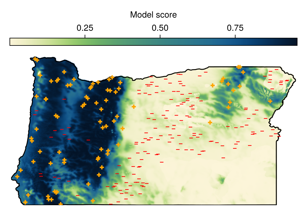
Code for the figure
f = Figure(; size = (500, 350))
ax = Axis(f[2, 1]; aspect = DataAspect())
hm = heatmap!(ax, Y; colormap = Reverse(:navia))
lines!(ax, landmass; color = :black)
scatter!(ax, model, color=labels(model), marker=[l ? :cross : :hline for l in labels(model)], colormap=[:red, :orange])
hidedecorations!(ax)
hidespines!(ax)
Colorbar(f[1, 1], hm; label = "Model score", vertical = false)
Calibrating the conformal classifier
train a conformal with alpha 0.05
conformal = train!(Conformal(0.05), model)Conformal{Float64}(0.05, 0.7093760271619234, 0.7614184562549292, true)apply conformal
present, absent, unsure, undetermined = predict(conformal, Y)Base.Generator{Vector{Set{Bool}}, SpeciesDistributionToolkit.var"#22#23"{Dict{Set{Bool}, SDMLayer{Bool}}}}(SpeciesDistributionToolkit.var"#22#23"{Dict{Set{Bool}, SDMLayer{Bool}}}(Dict{Set{Bool}, SDMLayer{Bool}}(Set([0]) => 🗺️ A 517 × 990 layer (411406 Bool cells), Set([1]) => 🗺️ A 517 × 990 layer (411406 Bool cells), Set() => 🗺️ A 517 × 990 layer (411406 Bool cells), Set([0, 1]) => 🗺️ A 517 × 990 layer (411406 Bool cells))), Set{Bool}[Set([1]), Set([0]), Set([0, 1]), Set()])note that if we want to get a single outcome, for example only the unsure predictions, we can pass it as a final argument there
unsure = predict(conformal, Y, Set([true, false]))🗺️ A 517 × 990 layer with 411406 Bool cells
Spatial Reference System: +proj=longlat +datum=WGS84 +no_defsWe will turn this prediction into a polygon, which will help with some of the plotting we will do next:
uns = polygonize(unsure)MultiPolygon with 109 subpolygonsTurning layers into polygons is long
Not because this is a very hard problem – simply that because, for now, the code works, and it will work faster in a future release.
We can now visualize the part of the landscape where the model is confident about presence (dark green), where the outcome is uncertain (shaded area), and the areas where the model is certain about absence (light grey):
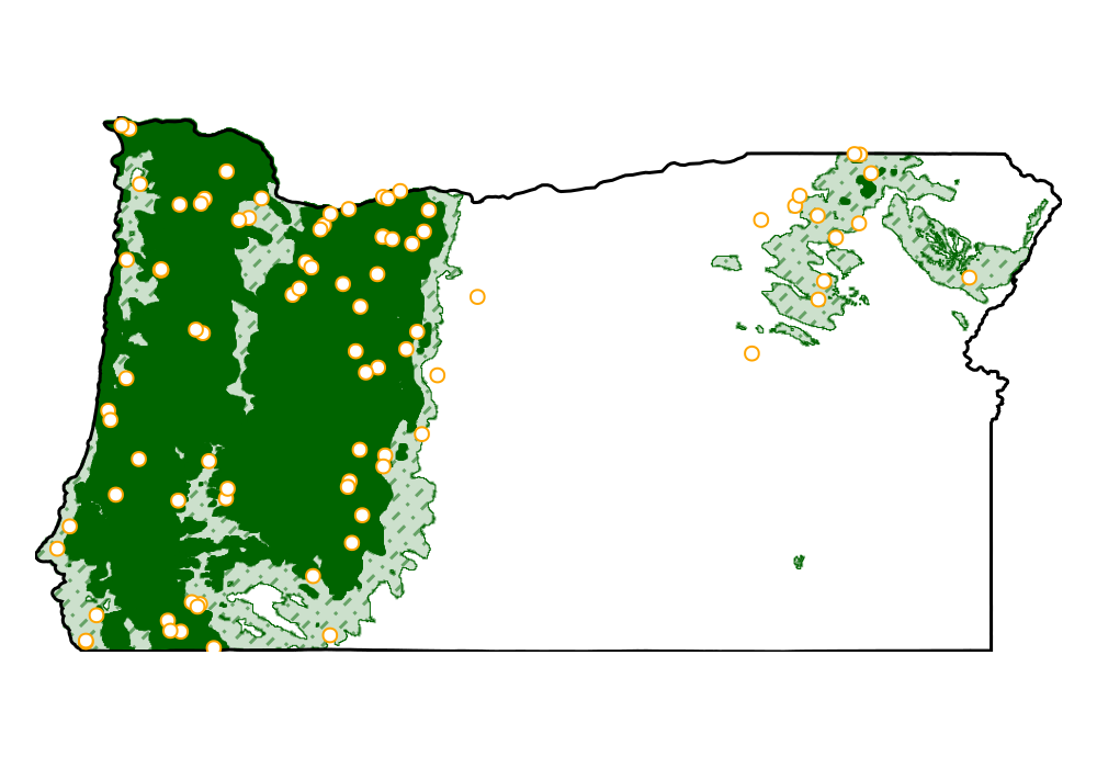
Code for the figure
f = Figure(; size = (500, 350))
ax = Axis(f[1, 1]; aspect = DataAspect())
heatmap!(ax, nodata(present, false); colormap = [:darkgreen])
poly!(ax, uns, color=:darkgreen, alpha=0.2)
lines!(ax, crosshatch(uns; spacing=0.15, angle=45), color=:darkgreen, alpha=0.5, linestyle=:dashdot)
lines!(ax, uns, color=:darkgreen, linewidth=0.5)
lines!(ax, landmass; color = :black)
scatter!(ax, records; color = :white, strokecolor=:orange, strokewidth=1, markersize = 9)
hidedecorations!(ax)
hidespines!(ax)
Because the risk level α is set by the user, it is a good idea to change it, and measure how much of the area ends up associated to different types of predictions:
rls = LinRange(0.01, 0.15, 15)
rangesize = zeros(Float64, 4, length(rls))
A = cellarea(Y)
🗺️ A 517 × 990 layer with 411406 Float64 cells
Spatial Reference System: +proj=longlat +datum=WGS84 +no_defsStability of results
When looking at the effect of a parameter, it is useful to keep the same split of the data when measuring the response of the model. This ensures that the only thing that varies is the parameter itself. It is, similarly, a good idea to perform several replicates. Because we do none of these things here, the next figure will not display a smooth tendency.
We will do a simple loop to set the risk level, re-calibrate the conformal classifier, and then measure the range associated to each outcome:
for (i, rl) in enumerate(rls)
    risklevel!(conformal, rl)
    train!(conformal, model)
    pr, ab, un, ud = predict(conformal, Y)
    rangesize[1, i] += sum(mask(A, nodata(pr, false)))
    rangesize[2, i] += sum(mask(A, nodata(ab, false)))
    rangesize[3, i] += sum(mask(A, nodata(un, false)))
end
Because the surface is large, we will express the range in more reasonable units:
rangesize ./= 1e44×15 Matrix{Float64}:
5.82949 5.53846 5.59197 4.98685 5.41957 4.27792 4.60358 4.25624 5.23726 5.76974 4.95735 7.63867 7.65957 8.53579 10.7285
15.0155 14.5965 14.4958 14.9477 15.8581 14.8823 15.9176 15.1201 16.5012 14.6903 15.4484 15.1404 14.435 13.9086 13.7896
4.58594 5.29593 5.3432 5.49634 4.15326 6.27069 4.90975 6.05456 3.69246 4.97086 5.0252 2.6519 3.33637 2.98652 0.912905
0.0 0.0 0.0 0.0 0.0 0.0 0.0 0.0 0.0 0.0 0.0 0.0 0.0 0.0 0.0And now, we can plot:
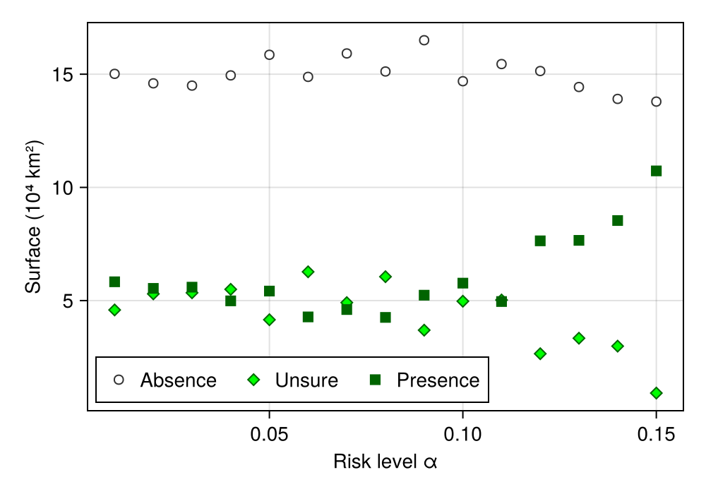
Code for the figure
f = Figure(; size = (500, 350))
ax = Axis(f[1, 1]; ylabel = "Surface (10⁴ km²)", xlabel = "Risk level α")
scatter!(ax, rls, rangesize[2, :]; label = "Absence", color=:white, strokecolor=:grey20, strokewidth=1)
scatter!(ax, rls, rangesize[3, :]; label = "Unsure", color=:lime, strokecolor=:darkgreen, strokewidth=1, marker=:diamond)
scatter!(ax, rls, rangesize[1, :]; label = "Presence", color=:darkgreen, marker=:rect, markersize=12)
axislegend(ax; position = :lb, nbanks = 3)
Continuous estimate of uncertainty
In this section, we will rely on conformal prediction and boostrapping to provide a more quantitative estimate of outcome uncertainty.
This is not best practice
Nothing that follows is a published technique, or even a particularly well tested idea. This section is included for the purpose of (i) notetaking, as this may be an idea worth exploring, and (ii) illustrating how the package can be used to do new things relatively easily.
We start by wrapping our model into a bagged ensemble of 50 sub-models:
bagged = Bagging(model, 50)
train!(bagged)
{RawData → Logistic → P(x) ≥ 0.263} × 50We will re-calibrate the conformal predictor (we previously changed it when estimating the range):
risklevel!(conformal, 0.05)
train!(conformal, model)
Conformal{Float64}(0.05, 0.7778942862772134, 0.8655201641769286, true)Because the bagged model is an homogenous ensemble, we can write our own consensus function to aggregate the outcome of each of the models in the ensemble. What we are after is, simply put, the proportion of models that, when passed to the conformal predictor, return a decision of "ambiguous", i.e. they can support both the true and false outcome.
isunsure = (x) -> count(isequal(Set([true, false])), predict(conformal, x))/length(x)#5 (generic function with 1 method)With this function written, we can get the summary of how many models return the unsure decision, for each point in the layer:
B = predict(bagged, L; threshold = false, consensus = isunsure)🗺️ A 517 × 990 layer with 411406 Float64 cells
Spatial Reference System: +proj=longlat +datum=WGS84 +no_defsAnd we can finally plot this model, in order to identify areas where most of the predictions are uncertain:
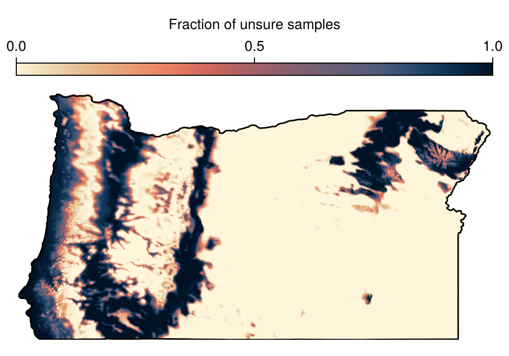
Code for the figure
f = Figure(; size = (500, 350))
ax = Axis(f[2, 1]; aspect = DataAspect())
hm = heatmap!(ax, B; colormap = Reverse(:lipari))
lines!(ax, landmass; color = :black)
Colorbar(f[1, 1], hm; label = "Fraction of unsure samples", vertical = false)
hidedecorations!(ax)
hidespines!(ax)
Related documentation
SDeMo.Conformal Type
ConformalThis objects wraps values for conformal prediction. It has a risk level α, and a threshold for the positive and negative classes, resp. q₊ and q₋. In the case of regular CP, the two thresholds are the same. For Mondrian CP, they are different.
This type has a trained flag and therefore supports the istrained function. If the prediction is attempted with a model that has not been trained, it should result in an UntrainedModelError.
SDeMo.risklevel Function
risklevel(cp::Conformal)Returns the risk level of the conformal predictor.
sourceSDeMo.risklevel! Function
risklevel!(cp::Conformal, α::T) where {T <: AbstractFloat}Changes the risk level of the conformal predictor. It will need to be recalibrated.
sourceSimpleSDMLayers.cellarea Function
cellarea(layer::T; R = 6371.0)Returns the area of each cell in km², assuming a radius of the Earth or R (in km). This is only returned for layers in WGS84, which can be forced with interpolate.
References
- Poisot, T. (Dec 2025). Conformal prediction quantifies the uncertainty of species distribution models. Publisher: EcoEvoRxiv.