Introduction
Community ecologists are fascinated by counting things. It is therefore no surprise that early food web research paid so much attention to counting species, counting trophic links, and uncovering the relationship that binds them – and it is undeniable that these inquiries kickstarted what is now one of the most rapidly growing fields of ecology (Borrett, Moody, and Edelmann 2014). More species (S) always means more links (L); this scaling is universal and appears both in observed food webs and under purely neutral models of food web structure (Canard et al. 2012). In fact, these numbers underlie most measures used to describe food webs (Delmas et al. 2018). The structure of a food web, in turn, is almost always required to understand how the community functions, develops, and responds to changes (McCann 2012; Thompson et al. 2012), to the point where some authors suggested that describing food webs was a necessity for community ecology (McCann 2007; Seibold et al. 2018). To this end, a first step is to come up with an estimate for the number of existing trophic links, through sampling or otherwise. Although both L and S can be counted in nature, the measurement of links is orders of magnitude more difficult than the observation of species (P. Jordano 2016a, 2016b). As a result, we have far more information about values of S. In fact, the distribution of species richness across the world is probably the most frequently observed and modelled ecological phenomenon. Therefore, if we can predict L from S in an ecologically realistic way, we would be in a position to make first order approximations of food web structure at large scales, even under our current data-limited regime.
Measures of food web structure react most strongly to a handful of important quantities. The first and most straightforward is L, the number of trophic links among species. This quantity can be large, especially in species-rich habitats, but it cannot be arbitrarily large. It is clear to any observer of nature that of all imaginable trophic links, only a fraction actually occur. If an ecological community contains S species, then the maximum number of links in its food web is S2: a community of omnivorous cannibals. This leads to the second quantity: a ratio called connectance and defined by ecologists as Co = L/S2. Connectance has become a fundamental quantity for nearly all other measures of food web structure and dynamics (Pascual and Dunne 2006). The third important quantity is another ratio: linkage density, LD = L/S. This value represents the number of links added to the network for every additional species in the ecological system. A closely related quantity is LD × 2, which is the average degree: the average number of species with which any taxa is expected to interact, either as predator or prey. These quantities capture ecologically important aspects of a network, and all can be derived from the observation or prediction of L links among S species.
Because L represents such a fundamental quantity, many predictive models have been considered over the years. Here we describe three popular approaches before describing our own proposed model. The link-species scaling (LSSL) (Cohen and Briand 1984) assumes that all networks have the same average degree; that is, most species should have the same number of links. Links are modelled as the number of species times a constant:
LLSSL = b × S
(1)
with b ≈ 2. This model imagines that every species added to a community increases the number of links by two – for example, an animal which consumes one resource and is consumed by one predator. This model started to show its deficiencies when data on larger food webs became available: in these larger webs, L increased faster than a linear function of S. Perhaps then all networks have the same connectance (Martinez 1992)? In other words, a food web is always equally filled, regardless of whether it has 5 or 5000 species. Under the so-called “constant connectance” model, the number of links is proportional to the richness squared,
LCC = b × S2 ,
(2)
where b is a constant in ]0, 1[ representing the expected value of connectance. The assumption of a scaling exponent of 2 can be relaxed (Martinez 1992), so that L is not in direct proportion to the maximum number of links:
LPL = b × Sa .
(3)
This “power law” model can be parameterized in many ways, including spatial scaling and species area relationships (Brose et al. 2004). It is also a general case of the previous two models, encompassing both link-species scaling (a = 1, b ≈ 2) and the strict constant connectance (a = 2, 0 < b < 1) depending on which parameters are fixed. Power laws are very flexible, and indeed this function matches empirical data well – so well that it is often treated as a “true” model which captures the scaling of link number with species richness (Winemiller et al. 2001; Garlaschelli, Caldarelli, and Pietronero 2003; Riede et al. 2010), and from which we should draw ecological inferences about what shapes food webs. However, this approach is limited, because the parameters of a power law relationship can arise from many mechanisms, and are difficult to reason about ecologically.
But the question of how informative parameters of a power law can be is moot. Indeed, both the general model and its variants share an important shortcoming: they cannot be used for prediction while remaining within the bounds set by ecological principles. This has two causes. First, models that are variations of L ≈ b × Sa have no constraints – with the exception of the “constant connectance” model, in which Lcc has a maximum value of S2. However, we know that the number of links within a food web is both lower and upper bounded (Martinez 1992; Poisot and Gravel 2014): there can be no more than S2 links, and there can be no fewer than S − 1 links. This minimum of S − 1 holds for food webs in which all species interact – for example, a community of plants and herbivores where no plants are inedible and all herbivores must eat (Martinez 1992). Numerous simple food webs could have this minimal number of links – for example, a linear food chain wherein each trophic level consists of a single species, each of which consumes only the species below it; or a grazing herbivore which feeds on every plant in a field. Thus the number of links is constrained by ecological principles to be between S − 1 and S2, something which no present model includes. Secondly, accurate predictions of L from S are often difficult because of how parameters are estimated. This is usually done using a Gaussian likelihood for L, often after log transformation of both L and S. While this approach ensures that predicted values of L are always positive, it does nothing to ensure that they stay below S2 and above S − 1. Thus a good model for L should meet these two needs: a bounded expression for the average number of links, as well as a bounded distribution for its likelihood.
Here we suggest a new perspective for a model of L as a function of S which respects ecological bounds, and has a bounded distribution of the likelihood. We include the minimum constraint by modelling not the total number of links, but the number in excess of the minimum. We include the maximum constraint in a similar fashion to the constant connectance model described above, by modelling the proportion of flexible links which are realized in a community.
Interlude - deriving a process-based model for the number of links
Based on the ecological constraints discussed earlier, we know that the number of links L is an integer such that S − 1 ≤ L ≤ S2. Because we know that there are at least S − 1 links, there can be at most S2 − (S − 1) links in excess of this quantity. The S − 1 minimum links do not need to be modelled, because their existence is guaranteed as a pre-condition of observing the network. The question our model should address is therefore, how many of these S2 − (S − 1) “flexible” links are actually present? A second key piece of information is that the presence of a link can be viewed as the outcome of a discrete stochastic event, with the alternative outcome that the link is absent. We assume that all of these flexible links have the same chance of being realized, which we call p. Then, if we aggregate across all possible species pairs, the expected number of links is
LFL = p × [S2−(S−1)] + (S − 1) ,
(1)
where p ∈ [0, 1]. When p = 1, L is at its maximum (S2), and when p = 0 it is at the minimum value (S − 1). We use the notation LFL to represent that our model considers the number of “flexible” links in a food web; that is, the number of links in excess of the minimum but below the maximum.
Because we assume that every flexible link is an independent stochastic event with only two outcomes, we can follow recent literature on probabilistic ecological networks (Poisot, Cirtwill, et al. 2016) and represent them as independent Bernoulli trials with a probability of success p. This approach does not capture ecological mechanisms known to act on food webs (Petchey et al. 2008), but rather captures that any interaction is the outcome of many processes which can overall be considered probabilistic events (Poisot, Stouffer, and Gravel 2015). The assumption that flexible links can all be represented by Bernoulli events is an appropriate trade-off between biological realism and parameterization requirements.
Furthermore, the observation of L links in a food web represents an aggregation of S2 − (S − 1) such trials. If we then assume that p is a constant for all links in a particular food web, but may vary between food webs (a strong assumption which we later show is actually more stringent than what data suggest), we can model the distribution of links directly as a shifted beta-binomial variable:
$$ [L|S,\mu, \phi] = { S^2 - (S - 1) \choose L - (S - 1)} \frac{\mathrm{B}(L - (S - 1) + \mu \phi, S^2 - L + (1 - \mu)\phi)}{\mathrm{B}(\mu \phi, (1 - \mu)\phi)} $$
(2)
Where B is the beta function, μ is the average probability of a flexible link being realized (i.e. the average value of p across networks in the dataset) and ϕ is the concentration around this value. The support of this distribution is limited to only ecologically realistic values of L: it has no probability mass below S − 1 or above S2. This means that the problem of estimating values for μ and ϕ is reduced to fitting the univariate distribution described in eq. 2. For more detailed explanation of the model derivation, fitting, and comparison, see Experimental Procedures.
In this paper we will compare our flexible links model to three previous models for L. We estimate parameters and compare the performance of all models using open data from the mangal.io networks database (Poisot, Baiser, et al. 2016). This online, open-access database collects published information on all kinds of ecological networks, including 255 food webs detailing interactions between consumers and resources (Poisot et al. 2020). We use these data to show how our flexible links model not only outperforms existing efforts at predicting the number of links, but also has numerous desirable properties from which novel insights about the structure of food webs can be derived.
Results and Discussion
Flexible links model fits better and makes a plausible range of predictions
| Model | eq. | PSIS-LOO | ΔELPD | SEΔELPD |
|---|---|---|---|---|
| Flexible links | 1 | 2520.5 ± 44.4 | 0 | 0 |
| Power law (Brose et al. 2004) | 3 | 2564.3 ± 46.6 | -21.9 | 6.5 |
| Constant (Martinez 1992) | 2 | 2811.0 ± 68.3 | -145.3 | 21.1 |
| Link-species scaling (Cohen and Briand 1984) | 1 | 39840.1 ± 2795.1 | -18659.8 | 1381.7 |
When fit to the datasets archived on mangal.io, all four models fit without any problematic warnings (see Experimental Procedures), while our model for flexible links outperformed previous solutions to the problem of modelling L. The flexible links model, which we fit via a beta-binomial observation model, had the most favourable values of PSIS-LOO information criterion (table 1) and of expected log predictive density (ELPD), relative to the three competing models which used a negative binomial observation model. Pareto-smoothed important sampling serves as a guide to model selection (Vehtari, Gelman, and Gabry 2017); like other information criteria it approximates the error in cross-validation predictions. Smaller values indicate a model which makes better predictions. The calculation of PSIS-LOO can also provide some clues about potential model fits; in our case the algorithm suggested that the constant connectance model was sensitive to extreme observations. The expected log predictive density (ELPD), on the other hand, measures the predictive performance of the model; here, higher values indicate more reliable predictions (Vehtari, Gelman, and Gabry 2017). This suggests that the flexible links model will make the best predictions of L.
To be useful to ecologists, predictions of L must stay within realistic boundaries determined by ecological principles. We generated posterior predictions for all models and visualized them against these constraints (fig. 1). The LSSL model underestimates the number of links, especially in large networks: its predictions were frequently lower than the minimum S − 1. The constant connectance and power law models also made predictions below this value, especially for small values of S. The flexible links model made roughly the same predictions, but within ecologically realistic values.
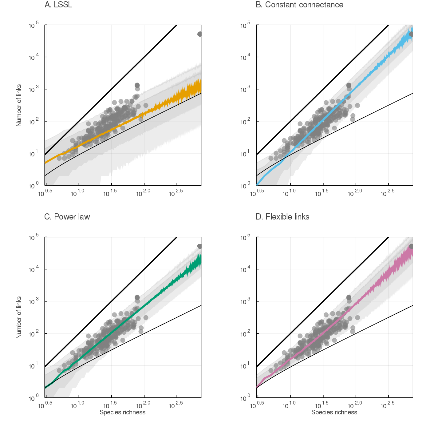
mangal.io database are plotted in each panel (grey dots), as well as the minimal S − 1 and maximal S2 number of links (thinner and bolder black lines, respectively). Predictions from the flexible links model are always plausible: they stay within these biological boundaries.The flexible links model makes realistic predictions for small communities
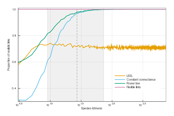
Constraints on food web structure are especially important for small communities. This is emphasized in fig. 2, which shows that all models other than the flexible links model fail to stay within realistic ecological constraints when S is small. The link-species scaling model made around 29% of unrealistic predictions of link numbers for every value of S (3 ≤ S ≤ 750). The constant connectance and power law models, on the other hand, also produced unrealistic results but for small networks only: more than 20% were unrealistic for networks comprising less than 12 and 7 species, respectively. Only the flexible links model, by design, never failed to predict numbers of links between S − 1 and S2. It must be noted that unrealistic predictions are most common in the shaded area of fig. 2, which represents 90% of the empirical data we used to fit the model; therefore it matters little that models agree for large S, since there are virtually no such networks observed.
Parameter estimates for all models
| Model | parameter | interpretation | value | SD |
|---|---|---|---|---|
| bS (Cohen and Briand 1984) | b | links per species | 2.2 | 0.047 |
| κ | concentration of L around mean | 1.4 | 0.12 | |
| bS2 (Martinez 1992) | b | proportion of links realized | 0.12 | 0.0041 |
| κ | concentration of L around mean | 4.0 | 0.37 | |
| bSa (Brose et al. 2004) | b | proportion of relationship | 0.37 | 0.054 |
| a | scaling of relationship | 1.7 | 0.043 | |
| κ | concentration of L around mean | 4.8 | 0.41 | |
| (S2 − (S − 1))p + S − 1 | μ | average value of p | 0.086 | 0.0037 |
| ϕ | concentration around value of μ | 24.3 | 2.4 |
Although we did not use the same approach to parameter estimation as previous authors, our approach to fitting these models recovered parameter estimates that are broadly congruent with previous works. We found a value of 2.2 for b of the LSSL model (table 2), which is close to the original value of approximately 2 (Cohen and Briand 1984). Similarly, we found a value of 0.12 for b of the constant connectance model, which was consistent with original estimates of 0.14 (Martinez 1992). Finally, the parameter values we found for the power law were also comparable to earlier estimates (Brose et al. 2004). All of these models were fit with a negative binomial observation model, which has an additional parameter, κ, which is sometimes called a “concentration” parameter. This value increases from the top of our table to the bottom, in the same sequence as predictive performance improves in table 1. This indicates that the model predictions are more concentrated around the mean predicted by the model (table 2, column 1).
Our parameter estimates for the flexible links model are ecologically meaningful. For large communities, our model should behave similarly to the constant connectance model and so it is no surprise that μ was about 0.09, which is close to our value of 0.12 for constant connectance. In addition, we obtained a rather large value of 24.3 for ϕ, which shrinks the variance around the mean of p to approximately 0.003 (var(p) = μ(1 − μ)/(1 + ϕ)). This indicates that food webs are largely similar in their probability of flexible links being realized (thus showing how our previous assumption that p might vary between food webs to be more conservative than strictly required). The flexible links model also uses fewer parameters than the power law model and makes slightly better predictions, which accounts for its superior performance in model comparison (table 1). In fig. S1, we compare the maximum a posteriori (MAP) estimates of our model parameters to their maximum likelihood estimates (MLE).
Connectance and linkage density can be derived from a model for links
Of the three important quantities which describe networks (L, Co and LD), we have directly modelled L only. However, we can use the parameter estimates from our model for L to parameterize a distribution for connectance (L/S2) and linkage density (L/S). We can derive this by noticing that eq. 1 can be rearranged to show how Co and LD are linear transformations of p:
$$ Co = \frac{L}{S^2} = p\left(1 - \frac{S-1}{S^2}\right) + \frac{S-1}{S^2} ,$$
(1)
and
$$ L_D = \frac{L}{S} = p \left(S - \frac{S-1}{S} \right) + \frac{S-1}{S},$$
(2)
For food webs with many species, these equations simplify: eq. 1 can be expressed as a second degree polynomial, LFL = p × S2 + (1 − p) × S + (p − 1), whose leading term is p × S2. Therefore, when S is large, eq. 1 and eq. 2 respectively approach Co = L/S2 ≈ p and LD = L/S ≈ pS. A study of eq. 1 and eq. 2 also provides insight into the ecological interpretation of the parameters in our equation. For example, eq. 2 implies that adding n species should increase the linkage density by approximately p × n. The addition of 11 new species (p − 1 according to table 2) should increase the linkage density in the food web by roughly 1, meaning that each species in the original network would be expected to develop 2 additional interactions. Similarly, eq. 1 shows that when S is large, we should expect a connectance which is a constant. Thus p has an interesting ecological interpretation: it represents the average connectance of networks large enough that the proportion (S − 1)/S2 is negligible.
Applications of the flexible links model to key food web questions
Our model is generative, and that is important and useful: we can use this model to correctly generate predictions that look like real data. This suggests that we can adapt the model, using either its parameters or predictions or both, to get a new perspective on many questions in network ecology. Here we show four possible applications that we think are interesting, in that relying on our model eliminates the need to speculate on the structure of networks, or to introduce new hypotheses to account for it.
Probability distributions for LD and Co
In a beta-binomial distribution, it is assumed that the probability of success p varies among groups of trials according to a Beta(μϕ, (1 − μ)ϕ) distribution. Since p has a beta distribution, the linear transformations described by eq. 1 and eq. 2 also describe beta distributions which have been shifted and scaled according to the number of species S in a community. This shows that just as L must be within ecologically meaningful bounds, Co (eq. 1) and LD (eq. 2) must be as well. The connectance of a food web is bounded by (S − 1)/S2 and 1, while the linkage density is bounded by (S − 1)/S and S.
We can convert the beta distribution for p into one for Co by replacing p with the transformation of Co as described above (eq. 1), and rescaling by the new range:
$$
[Co | S, \mu, \phi] = \frac{\left(Co - \frac{S-1}{S^2}\right)^{\mu \phi - 1}\left(1 - Co\right)^{(1 - \mu)\phi - 1} }{\left(1 - \frac{S-1}{S^2}\right)^{\phi - 1} \times \mathrm{B}(\mu \phi, (1 - \mu)\phi)}
$$
(3)
Similarly, we can convert the distribution for p into one for LD by replacing p with the transformation that gives LD (eq. 2)
$$
[L_{D} | S, \mu, \phi] = \frac{\left(L_D - \frac{S-1} {S}\right)^{\mu \phi - 1}\left(1 - L_D\right)^{(1 - \mu)\phi - 1} }{\left(S - \frac{S-1}{S}\right)^{\phi - 1} \times \mathrm{B}(\mu \phi, (1 - \mu)\phi)}
$$
(4)
In fig. 3, we show that the connectance and linkage density obtained from the equations above fit the empirical data well.
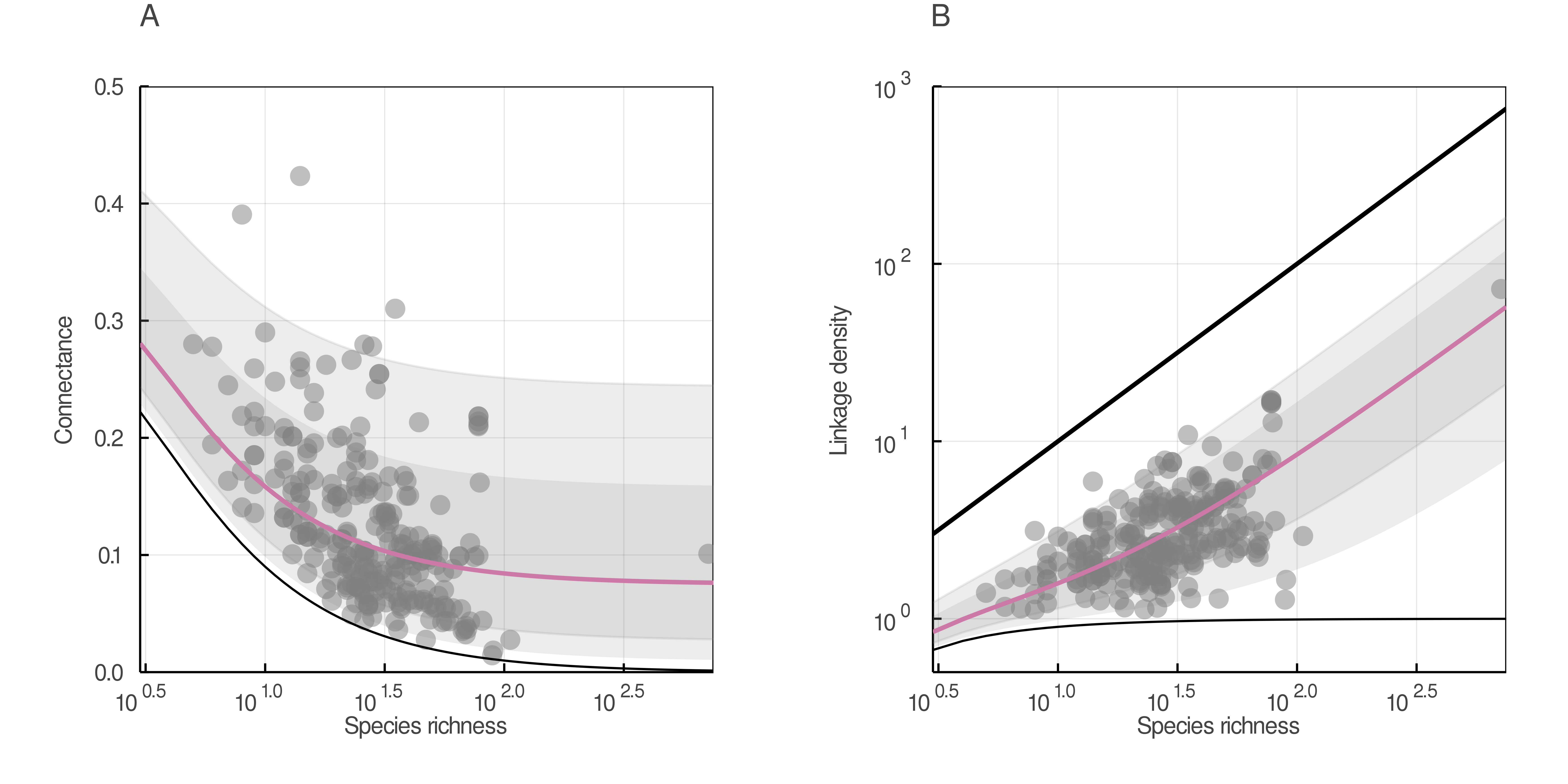
mangal.io database are plotted in each panel (grey dots). In A), the minimal (S − 1)/S2 connectance and in B) the minimal (S − 1)/S and maximum S linkage density are plotted (black lines).An analytic alternative to null-model testing
Ecologists are often faced with the issue of comparing several networks. A common question is whether a given network has an “unusual” number of links relative to some expectation. Traditionally these comparisons have been done by simulating a “null” distribution of random matrices (Fortuna and Bascompte 2006; Bascompte et al. 2003). This is intended to allow ecologists to compare food webs to a sort of standard, hopefully devoid of whatever biological process could alter the number of links. Importantly, this approach assumes that (i) connectance is a fixed property of the network, ignoring any stochasticity, and (ii) the simulated network distribution is an accurate and unbiased description of the null distribution. Yet recent advances in the study of probabilistic ecological networks show that the existence of links, and connectance itself is best thought of as a probabilistic quantity (Poisot, Cirtwill, et al. 2016). Given that connectance drives most of the measures of food web structure (Poisot and Gravel 2014), it is critical to have a reliable means of measuring differences from the expectation. We provide a way to assess whether the number of links in a network (and therefore its connectance) is surprising. We do so using maths rather than simulations.
The shifted beta-binomial can be approximated by a normal distribution with mean L̄ and variance σL2:
L ∼ Normal(L̄, σL2)
L̄ = (S2 − S + 1)μ + S − 1
$$\sigma_L^2 = (S^2 - S + 1) \mu (1 - \mu)(1 + \frac{S(S-1)}{\phi + 1})$$
(5)
This normal approximation is considered good whenever the skewness of the target distribution is modest. In food webs, this should be true whenever communities have more than about 10 species (see Experimental Procedures). This result means that given a network with observed species richness Sobs and observed links Lobs, we can calculate its z-score, i.e. how many standard deviations an observation is from the population average, as
$$z = \frac{L_{obs} - \bar{L}}{\sqrt{\sigma_L^2}} \,.$$
(6)
A network where L = L̄ will have a z-score of 0, and any network with more (fewer) links will have a positive (negative) z-score. Following this method, we computed the empirical z-scores for the 255 food webs archived on mangal.io (fig. 4). We found that 18 webs (7.1%) had a total number of observed links unusually higher than what was expected under the flexible links model (z> 1.96). These networks are interesting candidates for the study of mechanisms leading to high connectance.
Out of the 255 food webs, none was found to have an unusually low number of links (z< 1.96). In fact, z-scores this low are not possible in this dataset: food webs having the minimum value of S − 1 links are still within two standard deviations of the mean, for this sample. However, this sample contains the full diversity of food webs found in the mangal.io database. Hence, this does not mean that no food web will ever have a z-score lower than -1.96. If the flexible links model is fit to data from a specific system, food webs might have a surprisingly low number of links when compared to this population average. These networks would be interesting candidates for the study of mechanisms leading to low connectance or for the identification of under-sampled webs. Ecologists can thus use our method to assess the deviation of their own food webs from their random expectations.
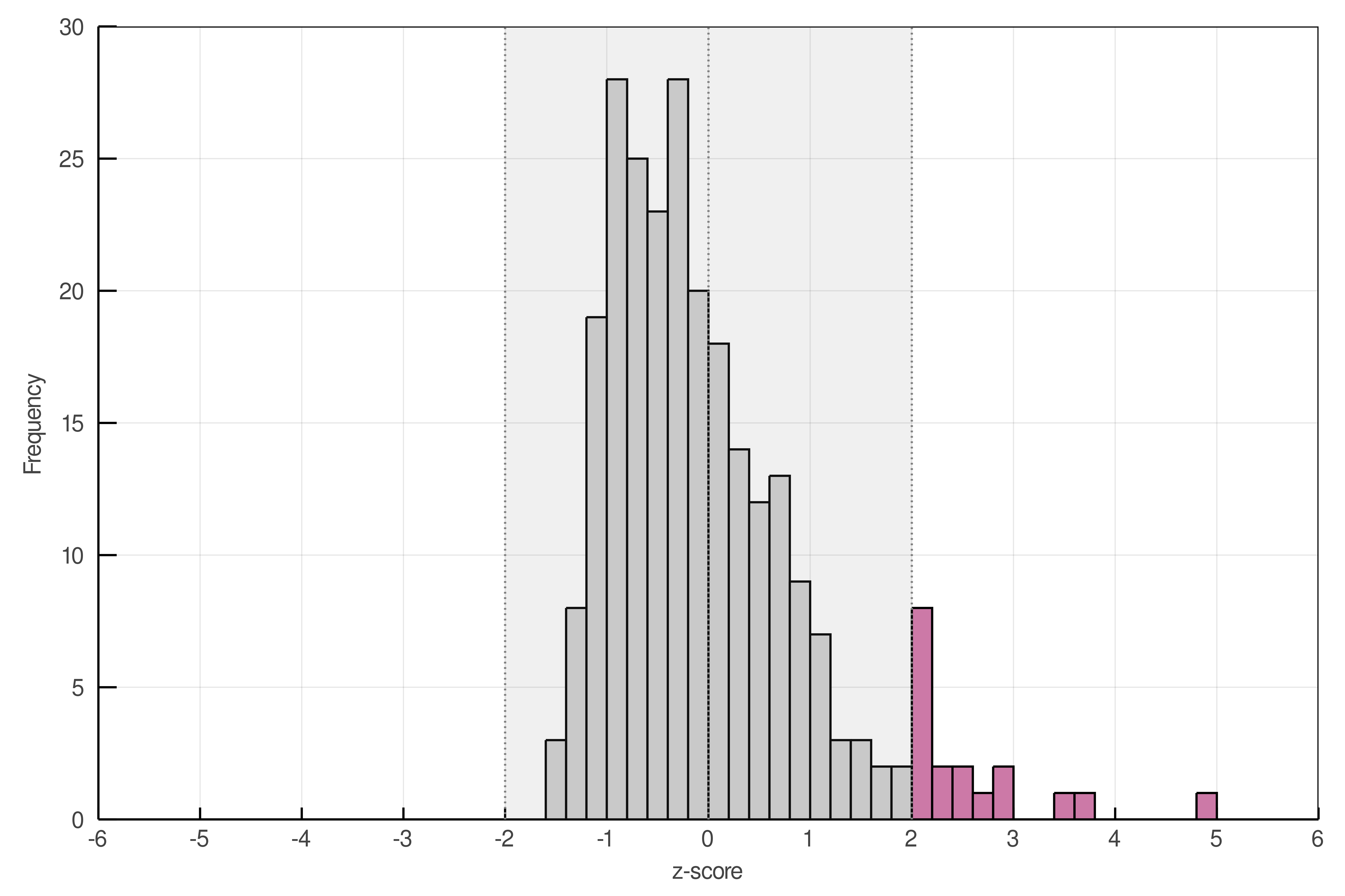
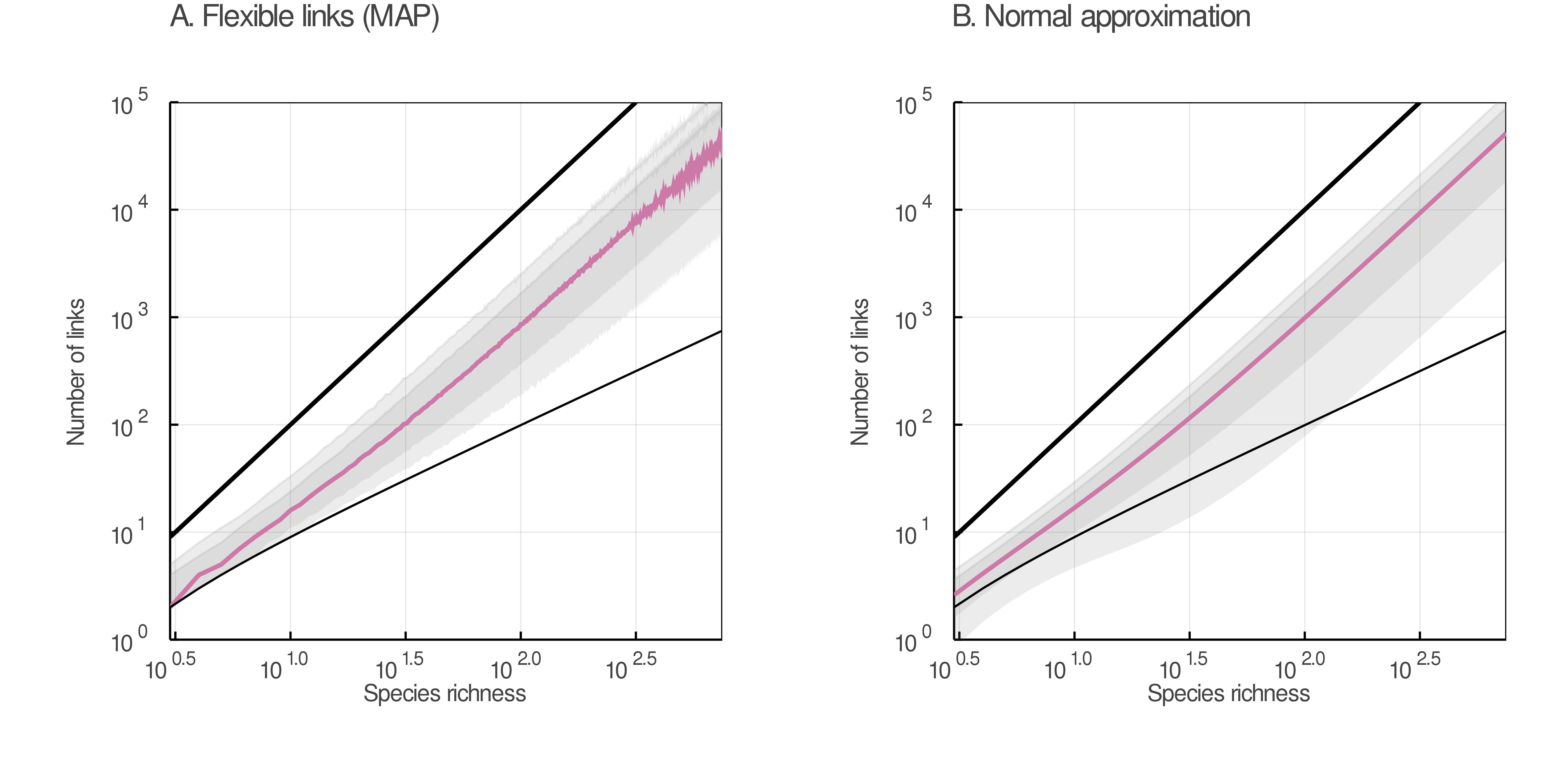
mangal.io have been computed using eq. 6. Food webs with an absolute z-score above 1.96 are in pink. The shaded region comprises all food webs with an absolute z-score below 1.96.In fig. 5, we show that the predictions made by the normal approximation (panel B) are similar to those made by the beta distribution parameterized with the maximum a posteriori values of μ and ϕ (panel A), although the former can undershoot the constraint on the minimum number of links. This undershooting, however, will not influence any actual z-scores, since no food webs have fewer than S − 1 links and therefore no z-scores so low can ever be observed.
We should see many different network-area relationships
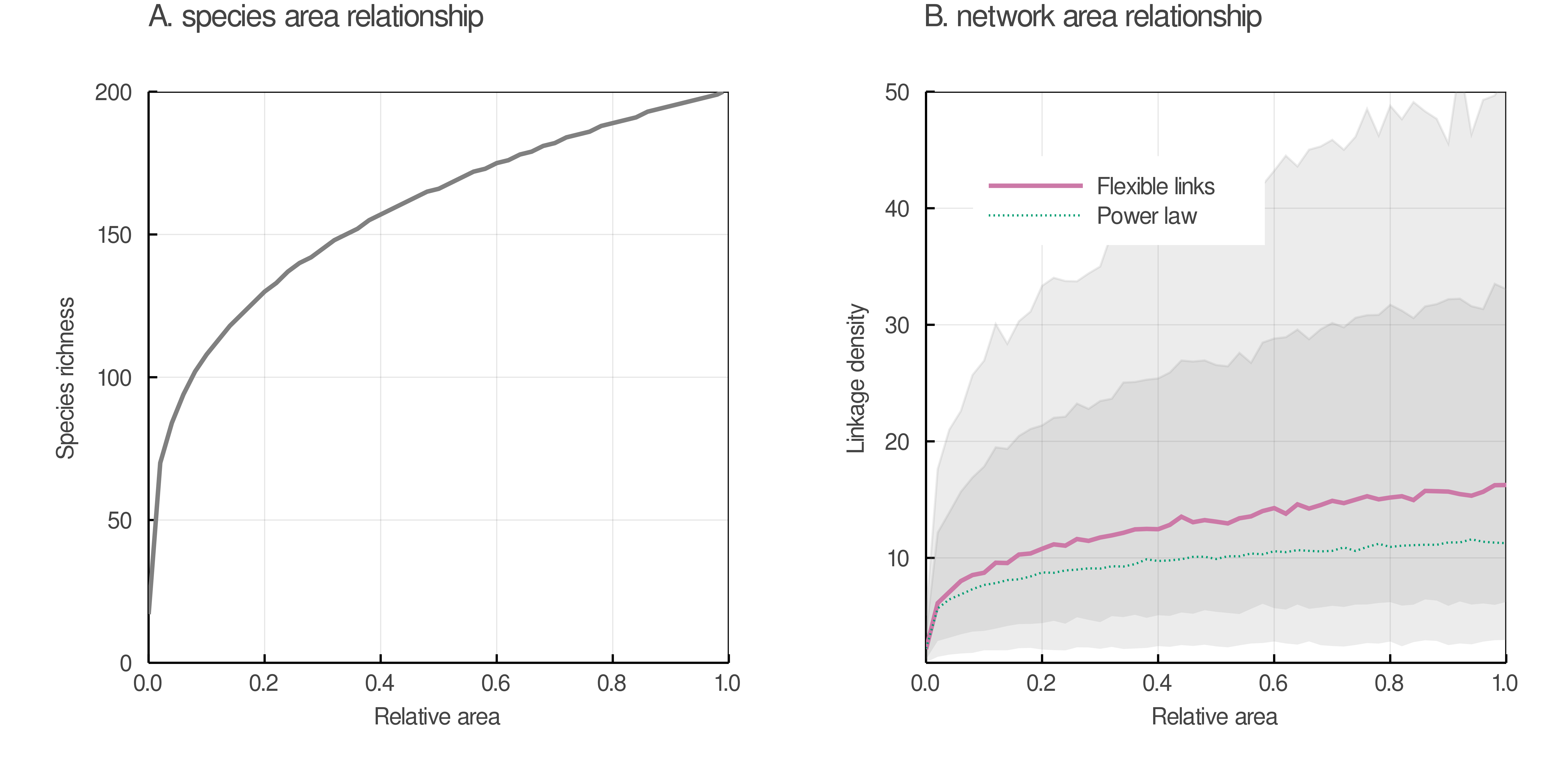
Our results bear important consequences for the nascent field of studying network-area relationships (NAR; Galiana et al. 2018). As it has long been observed that not all species in a food web diffuse equally through space (Holt et al. 1999), understanding how the shape of networks varies when the area increases is an important goal, and in fact underpins the development of a macroecological theory of food webs (Baiser et al. 2019). Using a power-law as the acceptable relationship between species and area (Dengler 2009; Williamson, Gaston, and Lonsdale 2001), the core idea of studying NAR is to predict network structure as a consequence of the effect of spatial scale on species richness (Galiana et al. 2018). Drawing on these results, we provide in fig. 6 a simple illustration of the fact that, due to the dispersal of values of L, the relationship between L/S and area can have a really wide confidence interval. While our posterior predictions generally match the empirical results on this topic (e.g. Wood et al. 2015), they suggest that we will observe many relationships between network structure and space, and that picking out the signal of network-area relationships might be difficult.
As of now, not many NARs have been documented empirically; but after the arguments made by Galiana et al. (2018) which tie the shape of these relationships to macroecological processes, we fully expect these relationships to be more frequently described moving forward. Our results suggest that our expectation of the amount of noise in these relationships should be realistic; while it is clear that these relationships exist, because of the scaling of dispersion in the number of links with the number of species, they will necessarily be noisy. Any described relationships will exist within extremely wide confidence intervals, and it might require a large quantity of empirical data to properly characterize them. As such, our model can help in assessing the difficulty of capturing some foundational relationships of food web structure.
Stability imposes a limit on network size
Can organisms really interact with an infinite number of partners? According to eq. 2, at large values of S, the linkage density scales according to p × S (which is supported by empirical data), and so species are expected to have on average 2 × p × S interactions. A useful concept in evolutionary biology is the “Darwinian demon” (Law 1979), i.e. an organism that would have infinite fitness in infinite environments. Our model seems to predict the emergence of what we call Eltonian demons, which can have arbitrarily large number of interactions. Yet we know that constraints on handling time of prey, for example, imposes hard limits on diet breadth (Forister and Jenkins 2017). This result suggests that there are other limitations to the size of food webs; indeed, the fact that L/S increases to worryingly large values only matters if ecological processes allow S to be large enough. It is known that food webs can get as high as energy transfer allows (Thompson et al. 2012), and as wide as competition allows (Kéfi et al. 2012). Furthermore, in more species-rich communities there is a greater diversity of functional traits among the interacting organisms; this limits interactions, because traits determine suitable interaction partners (Beckerman, Petchey, and Warren 2006; Bartomeus et al. 2016). In short, and as fig. 2 suggests, since food webs are likely to be constrained to remain within an acceptable richness, we have no reason to anticipate that p × S will keep growing infinitely.
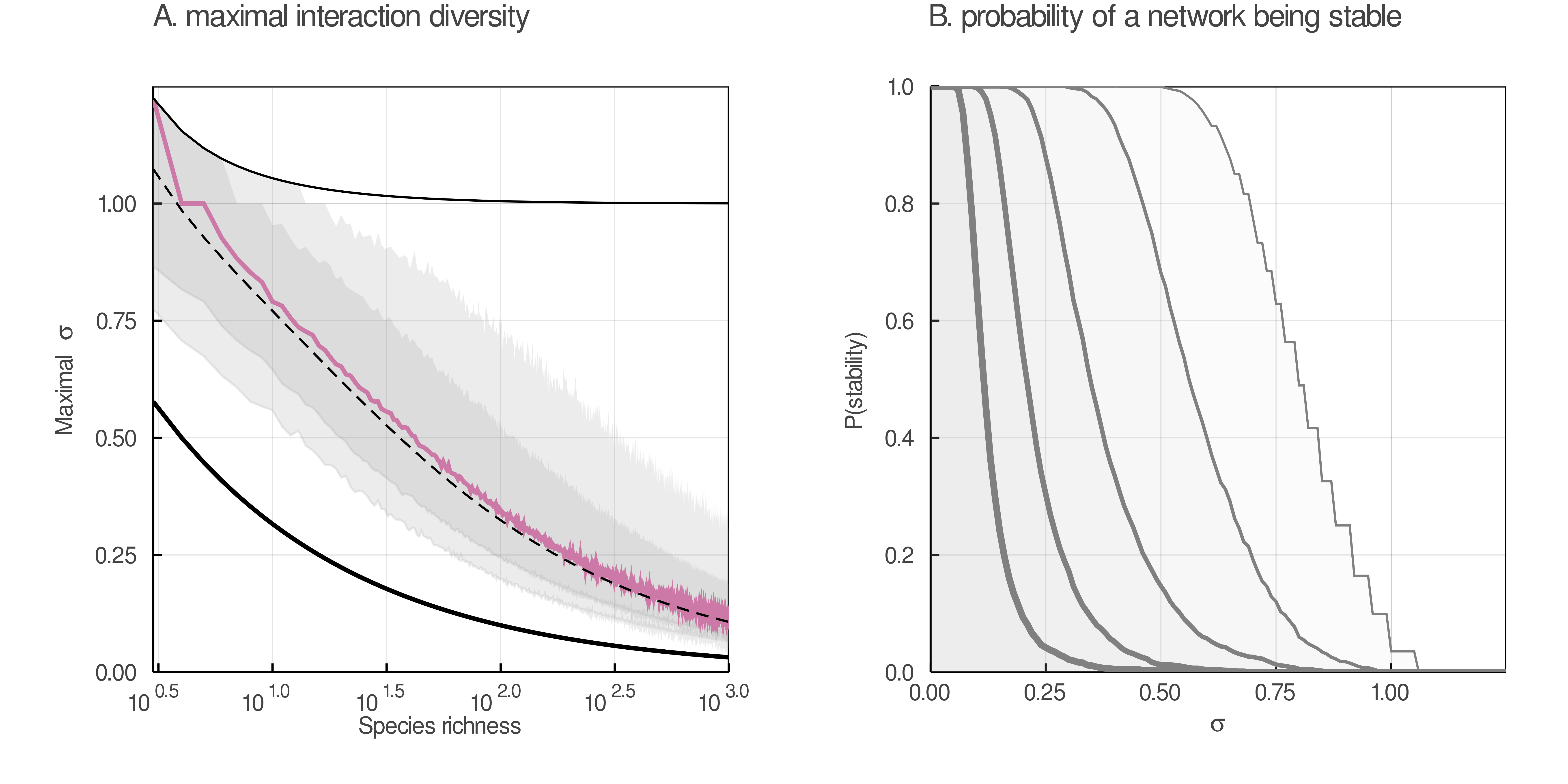
Network structure may itself prevent S from becoming large. May (May 1972) suggested that a network of richness S and connectance Co is stable as long as the criteria $\sigma \sqrt{S \times Co} < 1$ is satisfied, with σ being the standard deviation of the strengths of interactions. Although this criteria is not necessarily stringent enough for the stability of food webs (Allesina and Tang 2012, 2015), it still defines an approximate maximum value σ⋆ which is the value above which the system is expected to be unstable. This threshold is $\sigma^\star = 1/\sqrt{L_D}$, where LD is defined as in eq. 2. We illustrate this result in fig. 7, which reveals that σ⋆ falls towards 0 for larger species richness. The result in fig. 7 is in agreement with previous simulations, placing the threshold for stability at about 1200 species in food webs. These results show how ecological limitations, for example on connectance and the resulting stability of the system, can limit the size of food webs (Allesina and Tang 2012; Borrelli et al. 2015). In the second panel, we show that networks of increasing richness (thicker lines, varying on a log-scale from 101 to 103) have a lower probability of being stable, based on the proportion of stable networks in our posterior samples.
Conclusions
Here we derived eq. 1, a model for the prediction of the number of links in ecological networks using a beta-binomial distribution for L, and show how it outperforms previous and more commonly used models describing this relationship. More importantly, we showed that our model has parameters with a clear ecological interpretation (specifically, the value of p in eq. 1 is the expected value of the connectance when S is large), and makes predictions which remain within biological boundaries. There are a variety of “structural” models for food webs, such as the niche model (Williams and Martinez 2000), the cascade model (Cohen and Newman 1985), the DBM (Beckerman, Petchey, and Warren 2006) and ADBM (Petchey et al. 2008), the minimum potential niche model (Allesina, Alonso, and Pascual 2008), and the nested hierarchy model (Cattin et al. 2004) to name a few. All of these models make predictions of food web structure: based on some parameters (usually S and L, and sometimes vectors of species-level parameters) they output an adjacency matrix AS × S which contains either the presence or strength of trophic interactions. Therefore, these models require estimated values of L for a particular value of S, with the additional result that ∑A = L. Our approach can serve to improve the realism of these models, by imposing that the values of L they use are within realistic boundaries. For example, a common use of structural models is to generate a set of “null” predictions: possible values of A and L in the absence of the mechanism of interest. Empirical networks are then compared to this set of predictions, and are said to be significant if they are more extreme than 95% of the observations (Delmas et al. 2018). A challenge in this approach is that structural models may generate a wide range of predictions, including ecologically impossible values, leading a high false negative rate. This could be remedied by filtering this set of predictions according to our flexible links model, resulting in a narrower set of null predictions and a lower false negative rate. In general, our approach is complementary to other attempts to create ecologically-realistic food web models; for example, probabilistic models of the number of links per species which stay within ecological values (Kozubowski, Panorska, and Forister 2015).
This model also casts new light on previous results on the structure of food webs: small and large food webs behave differently (Garlaschelli, Caldarelli, and Pietronero 2003). Specifically, ecological networks most strongly deviate from scale free expectations when connectance is high (Dunne, Williams, and Martinez 2002). In our model, this behaviour emerges naturally: connectance increases sharply as species richness decreases (fig. 3) – that is, where the additive term (S − 1)/S2 in eq. 1 becomes progressively larger. In a sense, small ecological networks are different only due to the low values of S. Small networks have only a very limited number of flexible links, and this drives connectance to be greater. Connectance in turn has implications for many ecological properties. Connectance is more than the proportion of realized interactions. It has been associated with some of the most commonly used network measures (Poisot and Gravel 2014), and contains meaningful information on the stability (Dunne, Williams, and Martinez 2002; Montoya, Pimm, and Solé 2006) and dynamics (Vieira and Almeida‐Neto 2015) of ecological communities. A probability distribution for connectance not only accounts for the variability between networks, but can be used to describe fundamental properties of food webs and to identify ecological and evolutionary mechanisms shaping communities. A recent research direction has been to reveal its impact on resistance to invasion: denser networks with a higher connectance are comparatively more difficult to invade (Smith-Ramesh, Moore, and Schmitz 2016); different levels of connectance are also associated with different combinations of primary producers, consumers, and apex predators (Williams and Martinez 2000), which in turns determines which kind of species will have more success invading the network (Baiser, Russell, and Lockwood 2010). Because we can infer connectance from the richness of a community, our model also ties the invasion resistance of a network to its species richness.
The relationship between L and S has underpinned most of the literature on food web structure since the 1980s. Additional generations of data have allowed us to progress from the link-species scaling law, to constant connectance, to more general formulations based on a power law. Our model breaks with this tradition of iterating over the same family of relationships, and instead draws from our knowledge of ecological processes, and from novel tools in probabilistic programming. As a result, we provide predictions of the number of links which are closer to empirical data, stimulate new ecological insights, and can be safely assumed to always fall within realistic values. The results presented in fig. 6 (which reproduces results from Galiana et al. (2018)) and fig. 7 (which reproduces results from Allesina and Tang (2012)) may seem largely confirmatory; in fact, the ability of our model to reach the conclusions of previous milestone studies in food web ecology is a strong confirmation of its validity. We would like to point out that these approaches would usually require ecologists to make inferences not only on the parameters of interests, but also on the properties of a network for a given species richness. In contrast, our model allows a real economy of parameters and offers ecologists the ability to get several key elements of network structure for free if only the species richness is known.
Experimental Procedures
Availability of code and data
All code and data to reproduce this article is available at the Open Science Framework (DOI: 10.17605/OSF.IO/YGPZ2).
Bayesian model definitions
Generative models are flexible and powerful tools for understanding and predicting natural phenomena. These models aim to create simulated data with the same properties as observations. Creating such a model involves two key components: a mathematical expression which represents the ecological process being studied, and a distribution which represents our observations of this process. Both of these components can capture our ecological understanding of a system, including any constraints on the quantities studied.
Bayesian models are a common set of generative models, frequently used to study ecological systems. Here, we define Bayesian models for all 4 of the models described in eq. 1, eq. 2, eq. 3 and eq. 1. We use notation from Hobbs and Hooten (2015), writing out both the likelihood and the prior as a product over all 255 food webs in the mangal.io database.
Link-species scaling (LSSL) model:
$$
[b, \kappa | \textbf{L}, \textbf{S}] \propto \prod_{i = 1}^{255} \text{negative binomial}(L_i | b \times S_i, e^{\kappa}) \times \text{normal}(b|0.7, 0.02) \times \text{normal}(\kappa|2, 1)
$$
Constant connectance model:
$$
[b, \kappa | \textbf{L}, \textbf{S}] \propto \prod_{i = 1}^{255} \text{negative binomial}(L_i | b \times S_i^2, e^{\kappa}) \times \text{beta}(b|3, 7) \times \text{normal}(\kappa|2, 1)
$$
Power law model:
$$
[b, a, \kappa | \textbf{L}, \textbf{S}] \propto \prod_{i = 1}^{255} \text{negative binomial}(L_i | \exp(b) \times S_i^a, e^{\kappa}) \times \text{normal}(b| -3 , 1) \times \text{normal}(a | 2, 0.6) \times \text{normal}(\kappa|2, 1)
$$
Flexible links model:
$$
[\mu, \phi| \textbf{L}, \textbf{S}] \propto \prod_{i = 1}^{255} \text{beta binomial}(L_i - S_i + 1 | S_i^2 - S_i + 1, \mu \times e^{\phi}, (1 - \mu) \times e^\phi) \times \text{beta}(\mu| 3 , 7 ) \times \text{normal}(\phi | 3, 0.5)
$$
Note that while eϕ is shown in these equations for clarity, in the text we use ϕ to refer to the parameter after exponentiation. In the above equations, bold type indicates a vector of values; we use capital letters for L and S for consistency with the main text.
Because we want to compare all our models using information criteria, we were required to use a discrete likelihood to fit all models. Our model uses a discrete likelihood by default, but the previous three models (LSSL, constant connectance and the power law) normally do not. Instead, these models have typically been fit with Gaussian likelihoods, sometimes after log-transforming L and S. For example, eq. 3 becomes a linear relationship between log(L) and log(S). This ensures that predictions of L are always positive, but allows otherwise unconstrained variation on both sides of the mean. To keep this same spirit, we chose the negative binomial distribution for observations. This distribution is limited to positive integers, and can vary on both sides of the mean relationship.
We selected priors for our Bayesian models using a combination of literature and domain expertise. For example, we chose our prior distribution for p based on Martinez (1992) , who gave a value of constant connectance equal to 0.14. While the prior we use is “informative”, it is weakly so; as Martinez (1992) did not provide an estimate of the variance for his value we chose a relatively large variation around that mean. However, no information is available in the literature to inform a choice of prior for concentration parameters κ and ϕ. For these values, we followed the advice of Gabry et al. (2019) and performed prior predictive checks. Specifically, we chose priors that generated a wide range of values for Li, but which did not frequently predict webs of either maximum or minimum connectance, neither of which are observed in nature.
Explanation of shifted beta-binomial distribution
Equation eq. 1 implies that LFL has a binomial distribution, with S2 − S + 1 trials and a probability p of any flexible link being realized:
$$
[L | S, p] = { S^2 - (S - 1) \choose L - (S - 1)} p^{L-(S-1)}(1-p)^{S^2 - L} ,
$$
This is often termed a shifted binomial distribution.
We also note that ecological communities are different in many ways besides their number of species (S). Although we assume p to be fixed within one community, the precise value of p will change from one community to another. With this assumption, our likelihood becomes a shifted beta-binomial distribution:
$$
[L|S,\mu, \phi] = { S^2 - (S - 1) \choose L - (S - 1)} \frac{\mathrm{B}(L - (S - 1) + \mu \phi, S^2 - L + (1 - \mu)\phi)}{\mathrm{B}(\mu \phi, (1 - \mu)\phi)}
$$
(1)
Where B is the beta function. Thus, the problem of fitting this model becomes one of estimating the parameters of this univariate probability distribution.
Model fitting - data and software
We evaluated our model against 255 empirical food webs, available in the online database mangal.io (Poisot, Baiser, et al. 2016). We queried metadata (number of nodes and number of links) for all networks, and considered as food webs all networks having interactions of predation and herbivory. We use Stan (Carpenter et al. 2017) which implements Bayesian inference using Hamiltonian Monte Carlo. We ran all models using four chains and 2000 iterations per chain. In our figures we use the posterior predictive distribution, which is a distribution described by the model after conditioning on the data. There are numerous ways to display a probability distribution; here we have chosen to do so using the expectation (mean) and two arbitrary percentile intervals: 78% and 97%. These intervals were chosen based on the recommendations of McElreath (2020), and allowed us to capture most of the probability density in the tails of the posterior distributions.
Stan provides a number of diagnostics for samples from the posterior distribution, including R̂, effective sample size, and measures of effective tree depth and divergent iterations. None of these indicated problems with the posterior sampling. All models converged with no warnings; this indicates that is it safe to make inferences about the parameter estimates and to compare the models. However, the calculation of PSIS-LOO for the LSSL model warned of problematic values of the Pareto-k diagnostic statistic. This indicates that the model is heavily influenced by large values. Additionally, we had to drop the largest observation (> 50 000 links) from all datasets in order to calculate PSIS-LOO for the LSSL model. Taken together, this suggests that the LSSL model is insufficiently flexible to accurately reproduce the data.
Normal approximation and analytic z-scores
We propose using a normal approximation to the beta-binomial distribution, to calculate analytic z-scores. This is based on a well-known similarity between the shape of a normal distribution and a binomial distribution. This approximation is considered good whenever the absolute skewness is less than 0.3 (Box, Hunter, and Hunter 2005), that is whenever:
$$
\frac{1}{\sqrt{S^2 - S + 1}}\left(\sqrt{\frac{1- \mu}{\mu}} - \sqrt{\frac{\mu}{1-\mu}}\right) < 0.3
$$
The beta-binomial distribution is close to the binomial distribution. The error in approximating the former with the latter is on the order of the inverse square of the parameter ϕ (Teerapabolarn 2014), which for our model is less than 0.0017.
Acknowledgments
We thank three anonymous reviewers, as well as Owen Petchey and Andrew Beckerman, for their helpful comments and suggestions. Funding was provided by the Institute for data valorization (IVADO) and the NSERC CREATE Computational Biodiversity Science and Services (BIOS2) training program. TP acknowledges funding from the John Evans Leaders’ funds from the Canadian Foundation for Innovation. This work was made possible thanks to the effort of volunteers developing high-quality free and open source software for research.
References
Allesina, S., D. Alonso, and M. Pascual. 2008. “A General Model for Food Web Structure.” Science 320 (5876): 658–61. https://doi.org/10.1126/science.1156269.
Allesina, Stefano, and Si Tang. 2012. “Stability Criteria for Complex Ecosystems.” Nature 483 (7388): 205–8. https://doi.org/10.1038/nature10832.
———. 2015. “The Stability–Complexity Relationship at Age 40: A Random Matrix Perspective.” Population Ecology 57 (1): 63–75. https://doi.org/10.1007/s10144-014-0471-0.
Baiser, Benjamin, Dominique Gravel, Alyssa R. Cirtwill, Jennifer A. Dunne, Ashkaan K. Fahimipour, Luis J. Gilarranz, Joshua A. Grochow, et al. 2019. “Ecogeographical Rules and the Macroecology of Food Webs.” Global Ecology and Biogeography 0 (0). https://doi.org/10.1111/geb.12925.
Baiser, Benjamin, Gareth J. Russell, and Julie L. Lockwood. 2010. “Connectance Determines Invasion Success via Trophic Interactions in Model Food Webs.” Oikos 119 (12): 1970–6. https://doi.org/10.1111/j.1600-0706.2010.18557.x.
Bartomeus, Ignasi, Dominique Gravel, Jason M. Tylianakis, Marcelo A. Aizen, Ian A. Dickie, and Maud Bernard‐Verdier. 2016. “A Common Framework for Identifying Linkage Rules Across Different Types of Interactions.” Functional Ecology 30 (12): 1894–1903. https://doi.org/10.1111/1365-2435.12666.
Bascompte, J., P. Jordano, C. J. Melian, and J. M. Olesen. 2003. “The Nested Assembly of Plant-Animal Mutualistic Networks.” Proceedings of the National Academy of Sciences 100 (16): 9383–7. https://doi.org/10.1073/pnas.1633576100.
Beckerman, Andrew P., Owen L. Petchey, and Philip H. Warren. 2006. “Foraging Biology Predicts Food Web Complexity.” Proceedings of the National Academy of Sciences 103 (37): 13745–9. https://doi.org/10.1073/pnas.0603039103.
Borrelli, Jonathan J., Stefano Allesina, Priyanga Amarasekare, Roger Arditi, Ivan Chase, John Damuth, Robert D. Holt, et al. 2015. “Selection on Stability Across Ecological Scales.” Trends in Ecology & Evolution 30 (7): 417–25. https://doi.org/10.1016/j.tree.2015.05.001.
Borrett, Stuart R., James Moody, and Achim Edelmann. 2014. “The Rise of Network Ecology: Maps of the Topic Diversity and Scientific Collaboration.” Ecological Modelling 293 (December): 111–27. https://doi.org/10.1016/j.ecolmodel.2014.02.019.
Box, George E. P., J. Stuart Hunter, and William Gordon Hunter. 2005. Statistics for Experimenters: Design, Innovation, and Discovery. Wiley-Interscience.
Brose, Ulrich, Annette Ostling, Kateri Harrison, and Neo D. Martinez. 2004. “Unified Spatial Scaling of Species and Their Trophic Interactions.” Nature 428 (6979): 167–71. https://doi.org/10.1038/nature02297.
Canard, Elsa, Nicolas Mouquet, Lucile Marescot, Kevin J. Gaston, Dominique Gravel, and David Mouillot. 2012. “Emergence of Structural Patterns in Neutral Trophic Networks.” PLOS ONE 7 (8): e38295. https://doi.org/10.1371/journal.pone.0038295.
Carpenter, Bob, Andrew Gelman, Matthew D. Hoffman, Daniel Lee, Ben Goodrich, Michael Betancourt, Marcus Brubaker, Jiqiang Guo, Peter Li, and Allen Riddell. 2017. “Stan: A Probabilistic Programming Language.” Journal of Statistical Software 76 (1): 1–32. https://doi.org/10.18637/jss.v076.i01.
Cattin, Marie-France, Louis-Félix Bersier, Carolin Banašek-Richter, Richard Baltensperger, and Jean-Pierre Gabriel. 2004. “Phylogenetic Constraints and Adaptation Explain Food-Web Structure.” Nature 427 (6977): 835–39. https://doi.org/10.1038/nature02327.
Cohen, J. E., and F. Briand. 1984. “Trophic Links of Community Food Webs.” Proc Natl Acad Sci U S A 81 (13): 4105–9.
Cohen, Joel E., and Charles M. Newman. 1985. “A Stochastic Theory of Community Food Webs I. Models and Aggregated Data.” Proceedings of the Royal Society of London. Series B. Biological Sciences 224 (1237): 421–48. https://doi.org/10.1098/rspb.1985.0042.
Delmas, Eva, Mathilde Besson, Marie-Hélène Brice, Laura A. Burkle, Giulio V. Dalla Riva, Marie-Josée Fortin, Dominique Gravel, et al. 2018. “Analysing Ecological Networks of Species Interactions.” Biological Reviews, June, 112540. https://doi.org/10.1111/brv.12433.
Dengler, Jürgen. 2009. “Which Function Describes the Species–Area Relationship Best? A Review and Empirical Evaluation.” Journal of Biogeography 36 (4): 728–44. https://doi.org/10.1111/j.1365-2699.2008.02038.x.
Dunne, J. A., R. J. Williams, and N. D. Martinez. 2002. “Food-Web Structure and Network Theory: The Role of Connectance and Size.” Proceedings of the National Academy of Sciences 99 (20): 12917–22. https://doi.org/10.1073/pnas.192407699.
Forister, Matthew L., and Stephen H. Jenkins. 2017. “A Neutral Model for the Evolution of Diet Breadth.” The American Naturalist 190 (2): E40–E54. https://doi.org/10.1086/692325.
Fortuna, Miguel A., and Jordi Bascompte. 2006. “Habitat Loss and the Structure of Plant-Animal Mutualistic Networks: Mutualistic Networks and Habitat Loss.” Ecology Letters 9 (3): 281–86. https://doi.org/10.1111/j.1461-0248.2005.00868.x.
Gabry, Jonah, Daniel Simpson, Aki Vehtari, Michael Betancourt, and Andrew Gelman. 2019. “Visualization in Bayesian Workflow.” Journal of the Royal Statistical Society: Series A (Statistics in Society) 182 (2): 389–402. https://doi.org/10.1111/rssa.12378.
Galiana, Nuria, Miguel Lurgi, Bernat Claramunt-López, Marie-Josée Fortin, Shawn Leroux, Kevin Cazelles, Dominique Gravel, and José M. Montoya. 2018. “The Spatial Scaling of Species Interaction Networks.” Nature Ecology & Evolution 2 (5): 782–90. https://doi.org/10.1038/s41559-018-0517-3.
Garlaschelli, Diego, Guido Caldarelli, and Luciano Pietronero. 2003. “Universal Scaling Relations in Food Webs.” Nature 423 (6936): 165–68. https://doi.org/10.1038/nature01604.
Hobbs, N. Thompson, and Mevin B. Hooten. 2015. Bayesian Models: A Statistical Primer for Ecologists. Princeton, New Jersey: Princeton University Press.
Holt, Robert D., John H. Lawton, Gary A. Polis, and Neo D. Martinez. 1999. “Trophic Rank and the Species–Area Relationship.” Ecology 80 (5): 1495–1504. https://doi.org/10.1890/0012-9658(1999)080[1495:TRATSA]2.0.CO;2.
Jordano, Pedro. 2016a. “Sampling Networks of Ecological Interactions.” Edited by Daniel Stouffer. Functional Ecology 30 (12): 1883–93. https://doi.org/10.1111/1365-2435.12763.
———. 2016b. “Chasing Ecological Interactions.” PLOS Biol 14 (9): e1002559. https://doi.org/10.1371/journal.pbio.1002559.
Kéfi, Sonia, Eric L. Berlow, Evie A. Wieters, Sergio A. Navarrete, Owen L. Petchey, Spencer A. Wood, Alice Boit, et al. 2012. “More Than a Meal… Integrating Non-Feeding Interactions into Food Webs: More Than a Meal ….” Ecology Letters 15 (4): 291–300. https://doi.org/10.1111/j.1461-0248.2011.01732.x.
Kozubowski, Tomasz J., Anna K. Panorska, and Matthew L. Forister. 2015. “A Discrete Truncated Pareto Distribution.” Statistical Methodology 26 (September): 135–50. https://doi.org/10.1016/j.stamet.2015.04.002.
Law, Richard. 1979. “Optimal Life Histories Under Age-Specific Predation.” The American Naturalist 114 (3): 399–417. https://www.jstor.org/stable/2460187.
Martinez, Neo D. 1992. “Constant Connectance in Community Food Webs.” The American Naturalist 139 (6): 1208–18. http://www.jstor.org/stable/2462337.
May, Robert M. 1972. “Will a Large Complex System Be Stable?” Nature 238 (5364): 413–14. https://doi.org/10.1038/238413a0.
McCann, Kevin. 2007. “Protecting Biostructure.” Nature 446 (7131): 29–29. https://doi.org/10.1038/446029a.
McCann, Kevin S. 2012. Food Webs. Princeton: Princeton University Press.
McElreath, Richard. 2020. Statistical Rethinking: A Bayesian Course with Examples in R and STAN. CRC Press.
Montoya, José M., Stuart L. Pimm, and Ricard V. Solé. 2006. “Ecological Networks and Their Fragility.” Nature 442 (7100): 259–64. https://doi.org/10.1038/nature04927.
Pascual, Mercedes, and Jennifer A. Dunne. 2006. Ecological Networks: Linking Structure to Dynamics in Food Webs. Oxford University Press, USA.
Petchey, O. L., A. P. Beckerman, J. O. Riede, and P. H. Warren. 2008. “Size, Foraging, and Food Web Structure.” Proceedings of the National Academy of Sciences 105 (11): 4191–6. https://doi.org/10.1073/pnas.0710672105.
Poisot, Timothée, Benjamin Baiser, Jennifer A. Dunne, Sonia Kéfi, François Massol, Nicolas Mouquet, Tamara N. Romanuk, Daniel B. Stouffer, Spencer A. Wood, and Dominique Gravel. 2016. “Mangal - Making Ecological Network Analysis Simple.” Ecography 39 (4): 384–90. https://doi.org/10.1111/ecog.00976.
Poisot, Timothée, Gabriel Bergeron, Kevin Cazelles, Tad Dallas, Dominique Gravel, Andrew Macdonald, Benjamin Mercier, Clément Violet, and Steve Vissault. 2020. “Environmental Biases in the Study of Ecological Networks at the Planetary Scale.” bioRxiv, January, 2020.01.27.921429. https://doi.org/10.1101/2020.01.27.921429.
Poisot, Timothée, Alyssa R. Cirtwill, Kévin Cazelles, Dominique Gravel, Marie-Josée Fortin, and Daniel B. Stouffer. 2016. “The Structure of Probabilistic Networks.” Edited by Jana Vamosi. Methods in Ecology and Evolution 7 (3): 303–12. https://doi.org/10.1111/2041-210X.12468.
Poisot, Timothée, and Dominique Gravel. 2014. “When Is an Ecological Network Complex? Connectance Drives Degree Distribution and Emerging Network Properties.” PeerJ 2 (February): e251. https://doi.org/10.7717/peerj.251.
Poisot, Timothée, Daniel B. Stouffer, and Dominique Gravel. 2015. “Beyond Species: Why Ecological Interaction Networks Vary Through Space and Time.” Oikos 124 (3): 243–51. https://doi.org/10.1111/oik.01719.
Riede, Jens O., Björn C. Rall, Carolin Banasek-Richter, Sergio A. Navarrete, Evie A. Wieters, Mark C. Emmerson, Ute Jacob, and Ulrich Brose. 2010. “Chapter 3 - Scaling of Food-Web Properties with Diversity and Complexity Across Ecosystems.” In Advances in Ecological Research, edited by Guy Woodward, 42:139–70. Ecological Networks. Academic Press. https://doi.org/10.1016/B978-0-12-381363-3.00003-4.
Seibold, Sebastian, Marc W. Cadotte, J. Scott MacIvor, Simon Thorn, and Jörg Müller. 2018. “The Necessity of Multitrophic Approaches in Community Ecology.” Trends in Ecology & Evolution 33 (10): 754–64. https://doi.org/10.1016/j.tree.2018.07.001.
Smith-Ramesh, Lauren M., Alexandria C. Moore, and Oswald J. Schmitz. 2016. “Global Synthesis Suggests That Food Web Connectance Correlates to Invasion Resistance.” Global Change Biology, August, n/a–n/a. https://doi.org/10.1111/gcb.13460.
Teerapabolarn, K. 2014. “An Improved Binomial Approximation for the Beta Binomial Distribution.” International Journal of Pure and Apllied Mathematics 97 (4). https://doi.org/10.12732/ijpam.v97i4.10.
Thompson, Ross M., Ulrich Brose, Jennifer A. Dunne, Robert O. Hall, Sally Hladyz, Roger L. Kitching, Neo D. Martinez, et al. 2012. “Food Webs: Reconciling the Structure and Function of Biodiversity.” Trends in Ecology & Evolution 27 (12): 689–97. https://doi.org/10.1016/j.tree.2012.08.005.
Vehtari, Aki, Andrew Gelman, and Jonah Gabry. 2017. “Practical Bayesian Model Evaluation Using Leave-One-Out Cross-Validation and WAIC.” Statistics and Computing 27 (5): 1413–32. https://doi.org/10.1007/s11222-016-9696-4.
Vieira, Marcos Costa, and Mário Almeida‐Neto. 2015. “A Simple Stochastic Model for Complex Coextinctions in Mutualistic Networks: Robustness Decreases with Connectance.” Ecology Letters 18 (2): 144–52. https://doi.org/10.1111/ele.12394.
Williams, Richard J., and Neo D. Martinez. 2000. “Simple Rules Yield Complex Food Webs.” Nature 404 (6774): 180–83. https://doi.org/10.1038/35004572.
Williamson, Mark, Kevin J. Gaston, and W. M. Lonsdale. 2001. “The Species–Area Relationship Does Not Have an Asymptote!” Journal of Biogeography 28 (7): 827–30. https://doi.org/10.1046/j.1365-2699.2001.00603.x.
Winemiller, Kirk O., Eric R. Pianka, Laurie J. Vitt, and Anthony Joern. 2001. “Food Web Laws or Niche Theory? Six Independent Empirical Tests.” The American Naturalist 158 (2): 193–99. https://doi.org/10.1086/321315.
Wood, Spencer A., Roly Russell, Dieta Hanson, Richard J. Williams, and Jennifer A. Dunne. 2015. “Effects of Spatial Scale of Sampling on Food Web Structure.” Ecology and Evolution 5 (17): 3769–82. https://doi.org/10.1002/ece3.1640.