Arithmetic on layers

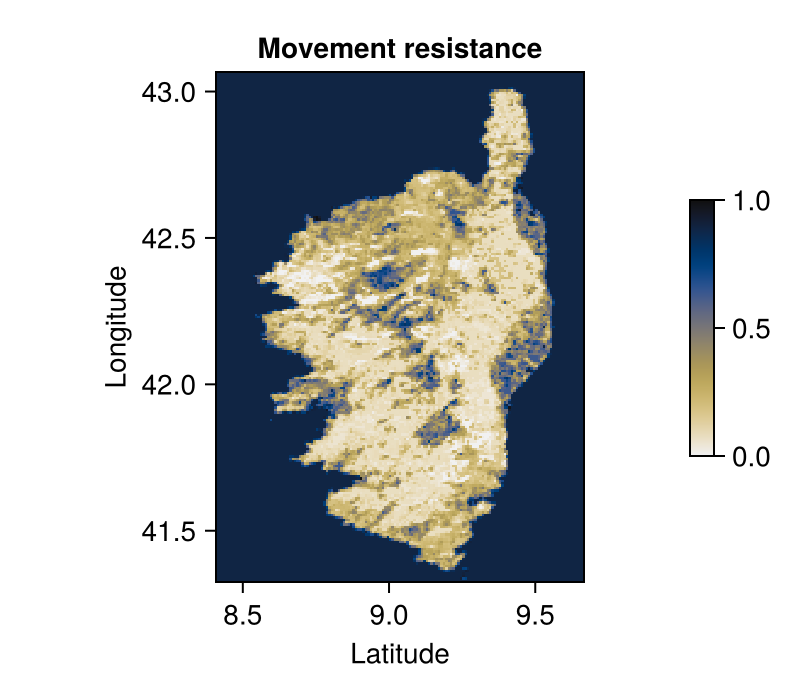
Layers can be manipulated as any other objects on which you can perform arithmetic. In other words, you can substract, add, multiply, and divide layers, either with other layers or with numbers. In this vignette, we will take a look at how this can facilitate the creation of a resistance map for functional connectivity analysis.

using SpeciesDistributionToolkit
using CairoMakie

We will work on the twelve classes of landcover provided by the EarthEnv data:

dataprovider = RasterData(EarthEnv, LandCover)

RasterData{EarthEnv, LandCover}(EarthEnv, LandCover)

In order to only read what is relevant to our illustration we will define a bounding box over Corsica.

spatial_extent = (left = 8.412, bottom = 41.325, right = 9.662, top = 43.060)

(left = 8.412, bottom = 41.325, right = 9.662, top = 43.06)

As a good practice, we check the names of the layers again. Note that checking the name of the layers will not download the data, so this may be a good time to remove some layers you are not interested in (which of course would not be a good idea for this specific application).

landcover_classes = SimpleSDMDatasets.layers(dataprovider)

12-element Vector{String}:
 "Evergreen/Deciduous Needleleaf Trees"
 "Evergreen Broadleaf Trees"
 "Deciduous Broadleaf Trees"
 "Mixed/Other Trees"
 "Shrubs"
 "Herbaceous Vegetation"
 "Cultivated and Managed Vegetation"
 "Regularly Flooded Vegetation"
 "Urban/Built-up"
 "Snow/Ice"
 "Barren"
 "Open Water"

To create a resistance map, we need to decide on a score for the resistance of each class of land use. For the sake of an hypothetical example, we will assume that the species we care about can easily traverse forested habitats, is less fond of shrubs, fields, etc., and is a poor swimmer who is afraid of cities. Think of it as your typical forestry graduate student.

classes_resistance = [0.1, 0.1, 0.1, 0.2, 0.4, 0.5, 0.7, 0.9, 1.2, 0.8, 1.2, 0.95]
classes_resistance = classes_resistance ./ sum(classes_resistance)

12-element Vector{Float64}:
 0.013986013986013988
 0.013986013986013988
 0.013986013986013988
 0.027972027972027975
 0.05594405594405595
 0.06993006993006994
 0.0979020979020979
 0.1258741258741259
 0.16783216783216784
 0.1118881118881119
 0.16783216783216784
 0.13286713286713286

The next step is to download the layers – we do so with a list comprehension, in order to get a vector of layers:

landuse = [
    SDMLayer(dataprovider; layer = class, full = true, spatial_extent...) for
    class in landcover_classes
];

The aggregation of the layers is simply ∑wᵢLᵢ, where wᵢ is the resistance of the i-th layer Lᵢ. In order to have the resistance layer expressed between 0 and 1, we finally call the rescale! method with new endpoints for the layer:

resistance_layer =
    reduce(.+, [landuse[i] .* classes_resistance[i] for i in eachindex(landuse)])
rescale!(resistance_layer)

SDM Layer with 31559 Float64 cells
	Proj string: +proj=longlat +datum=WGS84 +no_defs
	Grid size: (209, 151)

The remaining step is to visualize this resistance map, and add a little colorbar to show which areas will be more difficult to cross:

Code for the figure

resistance_map = heatmap(
    resistance_layer;
    colormap = Reverse(:linear_protanopic_deuteranopic_kbjyw_5_95_c25_n256),
    figure = (; size = (400, 350)),
    axis = (;
        aspect = DataAspect(),
        xlabel = "Latitude",
        ylabel = "Longitude",
        title = "Movement resistance",
    ),
)
Colorbar(resistance_map.figure[:, end + 1], resistance_map.plot; height = Relative(0.5))

This layer can then be used in landscape connectivity analyses using e.g. Omniscape.jl.