Layers and occurrence data

In this vignette, we will have a look at the ways in which occurrence data (from GBIF) and layer data can interact. In order to illustrate this, we will get information about the occurrences of Sitta whiteheadi, a species of bird endemic to Corsica. Finally, we will rely on the Phylopic package to download a silhouette of a bat to illustrate the figure.

using SpeciesDistributionToolkit
using CairoMakie
import Images
import Downloads

This sets up a bounding box for the region of interest:

spatial_extent = (left = 8.412, bottom = 41.325, right = 9.662, top = 43.060)

(left = 8.412, bottom = 41.325, right = 9.662, top = 43.06)

We will get our bioclimatic variable from CHELSA:

dataprovider = RasterData(CHELSA1, BioClim)

RasterData{CHELSA1, BioClim}(CHELSA1, BioClim)

The next step is to download the layers, making sure to correct the scale of the temperature (BIO1), which is multiplied by 10 in the CHELSA raw data:

temperature = 0.1SDMLayer(dataprovider; layer = "BIO1", spatial_extent...)
precipitation = SDMLayer(dataprovider; layer = "BIO12", spatial_extent...)

SDM Layer with 14432 Int16 cells
	Proj string: +proj=longlat +datum=WGS84 +no_defs
	Grid size: (209, 151)

Once we have the layer, we can grab the occurrence data from GBIF:

species = taxon("Sitta whiteheadi")
observations = occurrences(
    species,
    "decimalLatitude" => (spatial_extent.bottom, spatial_extent.top),
    "decimalLongitude" => (spatial_extent.left, spatial_extent.right),
    "limit" => 300,
    "occurrenceStatus" => "PRESENT",
)
while length(observations) < count(observations)
    occurrences!(observations)
end

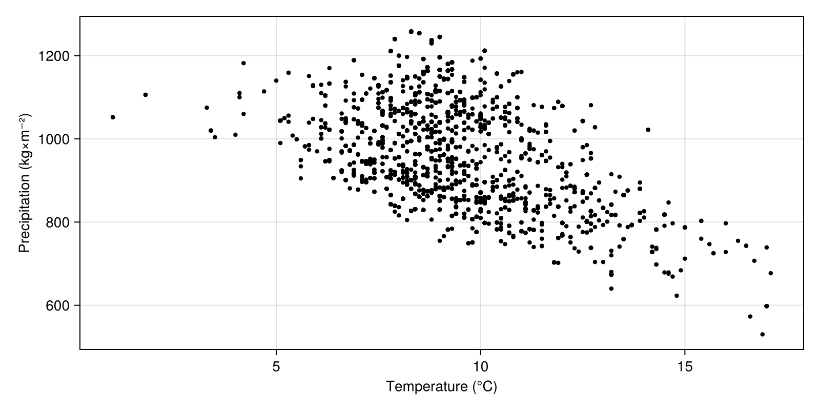
We can now setup a figure with the correct axes, and use the layer[occurrence] indexing method to extract the values from the layers at the location of each occurrence.

Code for the figure

figure = Figure(; size = (800, 400))
envirovars =
    Axis(figure[1, 1]; xlabel = "Temperature (°C)", ylabel = "Precipitation (kg×m⁻²)")
scatter!(envirovars, temperature[observations], precipitation[observations], markersize=6, color=:black)

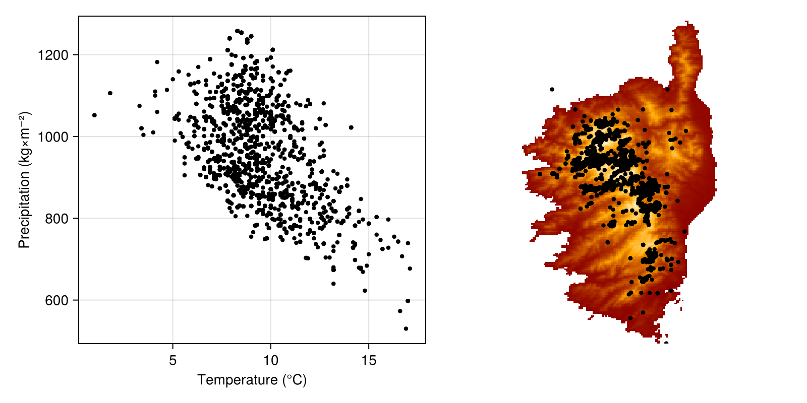
In order to also show these on the map, we will add a simple heatmap to the left of the figure, and overlay the points using longitudes and latitudes for the observations:

Code for the figure

spmap = Axis(figure[1, 2]; aspect = DataAspect())
hidedecorations!(spmap)
hidespines!(spmap)
heatmap!(spmap, temperature; colormap = :heat)
scatter!(spmap, observations; color = :black, markersize=6)

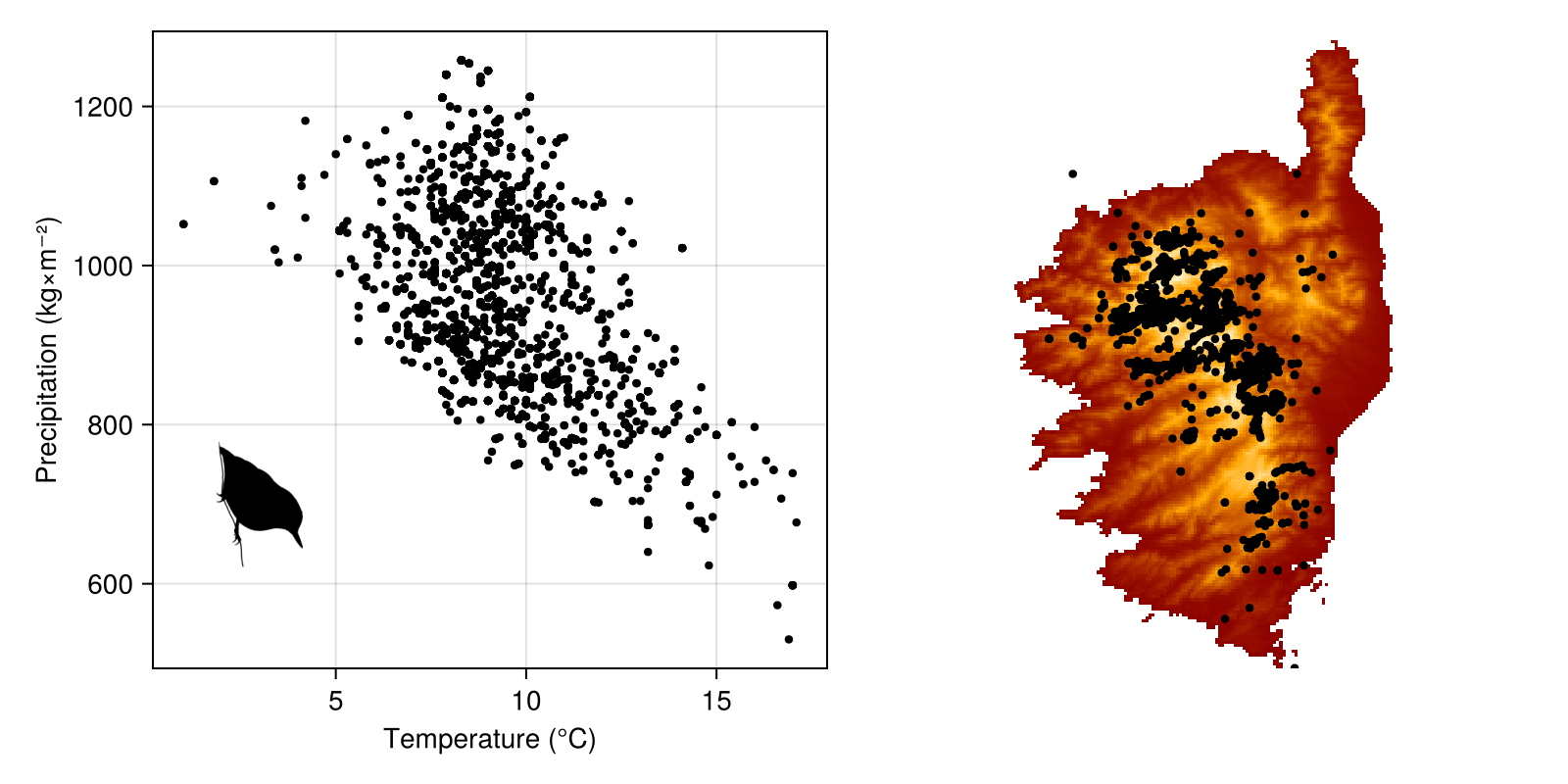
We can now add a silhouette of the species using Phylopic. We only want a single item here, and the search will by default be restricted to images that can be used with the least constraints. Note that we are searching using the GBIFTaxon object representing our species.

sp_uuid = Phylopic.imagesof(species; items = 1)

"Sitta carolinensis" => Base.UUID("4f24cf78-48d8-42ab-9e12-18853528c73c")

The next step is to get the url of the image – we are going to get the largest thumbnail (which is the default):

sp_thumbnail_url = Phylopic.thumbnail(sp_uuid)
sp_thumbnail_tmp = Downloads.download(sp_thumbnail_url)
sp_image = Images.load(sp_thumbnail_tmp)

Credit where credit is due!

The images on Phylopic are all created by volunteers. It is important to provide correct credit and attribution for their work. The attribution method will return the name of the creator and the correct license associated to this illustration:

Phylopic.attribution(sp_uuid)

Image of Sitta carolinensis provided by Andy Wilson

We can now use this image in a scatter plot – this uses the thumbnail as a scatter symbol, so we need to plot this like any other point. Because the thumbnail returned by default is rather large, we can rescale it based on the image size:

sp_size = Vec2f(reverse(size(sp_image) ./ 3))

2-element GeometryBasics.Vec{2, Float32} with indices SOneTo(2):
 64.0
 64.0

Finally, we can plot everything (note that the Phylopic images have a transparent background, so we are not hiding any information!):

Code for the figure

scatter!(envirovars, [3.0], [700.0]; marker = sp_image, markersize = sp_size)