Working with polygons

using SpeciesDistributionToolkit
using CairoMakie
import GeoJSON

In this tutorial, we will clip a layer to a polygon (in GeoJSON format), then use the same polygon to filter GBIF records.

About coordinates

GeoJSON coordinates are expressed in WGS84. For this reason, any polygon is assumed to be in this CRS, and all operations will be done by projecting the layer coordinates to this CRS.

We provide a very lightweight wrapper around the GADM database, which will return data as ready-to-use GeoJSON files.

DEU = SpeciesDistributionToolkit.gadm("DEU")

FeatureCollection with 1 Features

More about GADM

The only other function to interact with GADM is gadmlist, which takes either a series of places, as in

SpeciesDistributionToolkit.gadmlist("FRA", "Bretagne")

4-element Vector{String}:
 "Côtes-d'Armor"
 "Finistère"
 "Ille-et-Vilaine"
 "Morbihan"

or a level, to provide a list of places within a three-letter coded area at a specific depth:

SpeciesDistributionToolkit.gadmlist("FRA", 3)[1:3]

3-element Vector{String}:
 "Belley"
 "Bourg-en-Bresse"
 "Gex"

The next step is to get a layer, and so we will download the data about deciduous broadleaf trees from EarthEnv:

provider = RasterData(EarthEnv, LandCover)
layer = SDMLayer(
    provider;
    layer = "Deciduous Broadleaf Trees",
    left = 2.0,
    right = 20.0,
    bottom = 45.0,
    top = 57.0,
)

SDM Layer with 3110400 UInt8 cells
	Proj string: +proj=longlat +datum=WGS84 +no_defs
	Grid size: (1440, 2160)

We can check that this polygon is larger than the area we want:

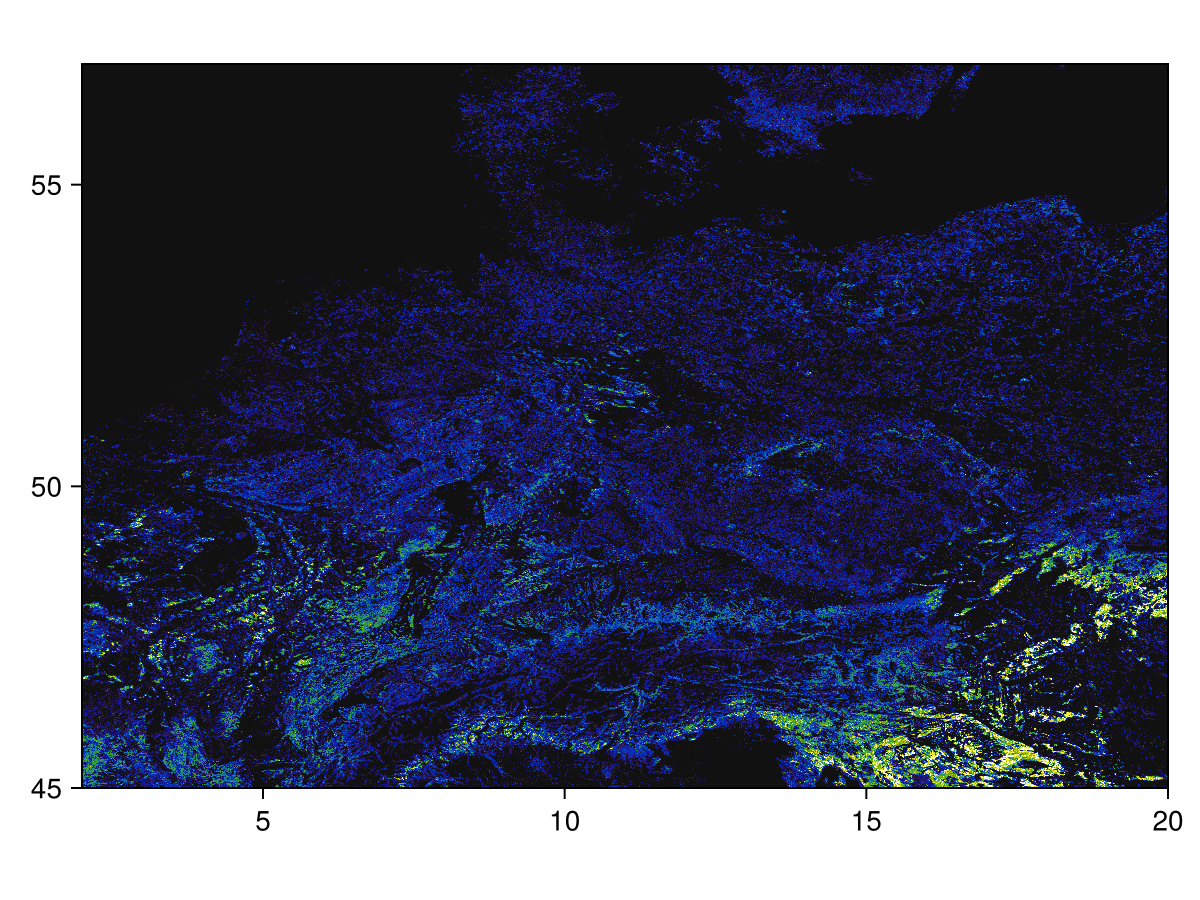
Code for the figure

heatmap(layer; colormap = :linear_kbgyw_5_98_c62_n256, axis = (; aspect = DataAspect()))

We can now mask this layer according to the polygon. This uses the same mask! method we use when masking with another layer:

mask!(layer, DEU)

SDM Layer with 661690 UInt8 cells
	Proj string: +proj=longlat +datum=WGS84 +no_defs
	Grid size: (1440, 2160)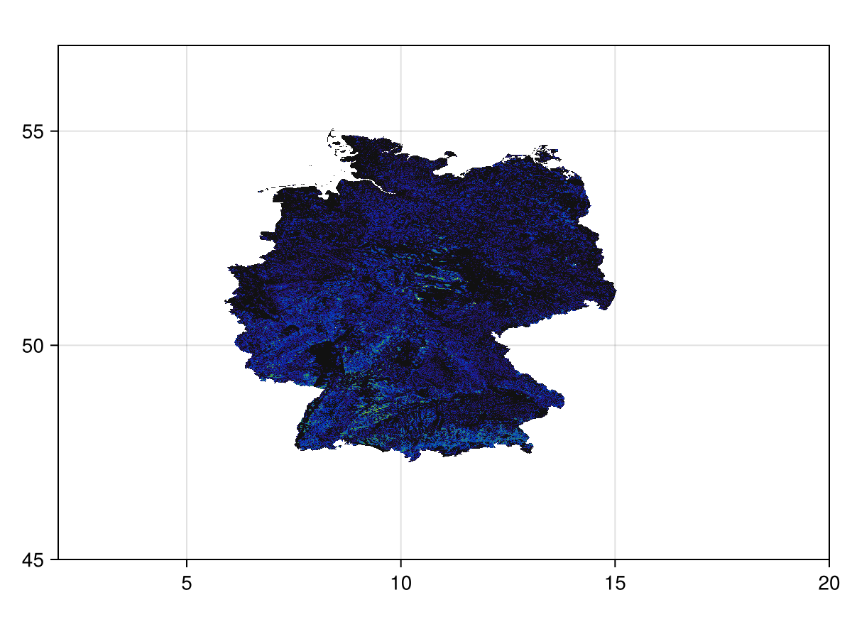

Code for the figure

heatmap(layer; colormap = :linear_kbgyw_5_98_c62_n256, axis = (; aspect = DataAspect()))

This is a much larger layer than we need! For this reason, we will trim it so that the empty areas are removed:

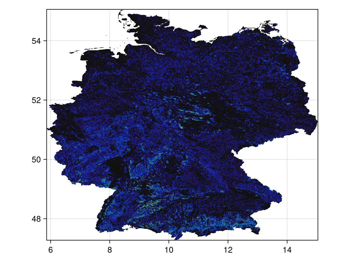
Code for the figure

heatmap(
    trim(layer);
    colormap = :linear_kbgyw_5_98_c62_n256,
    axis = (; aspect = DataAspect()),
)

Let's now get some occurrences in the area defined by the layer boundingbox:

sp = taxon("Eliomys quercinus")
presences = occurrences(
    sp,
    trim(layer),
    "occurrenceStatus" => "PRESENT",
    "limit" => 300,
)
while length(presences) < count(presences)
    occurrences!(presences)
end

Occurrences from a layer

The GBIF.occurrences method can accept a layer as its second argument, to limit to the occurrence of a species within the bounding box of this layer. If a layer is used as the sole argument, all occurrences in the bounding box are queried.

We can plot the layer and the occurrences we have retrieved so far:

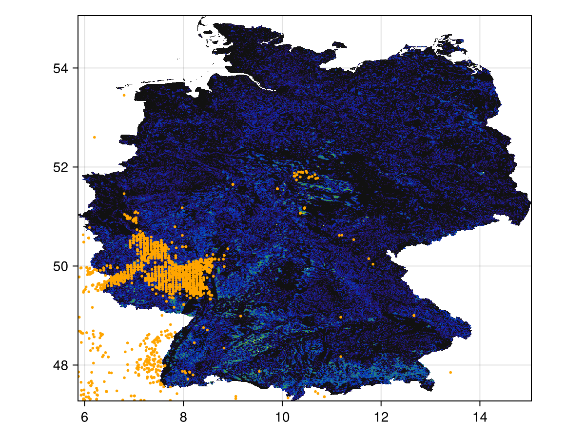
Code for the figure

heatmap(
    trim(layer);
    colormap = :linear_kbgyw_5_98_c62_n256,
    axis = (; aspect = DataAspect()),
)
scatter!(presences; color = :orange, markersize = 4)

Some of these occurrences are outside of the masked region in the layer. For this reason, we will use the non-mutating mask method on the GBIF records:

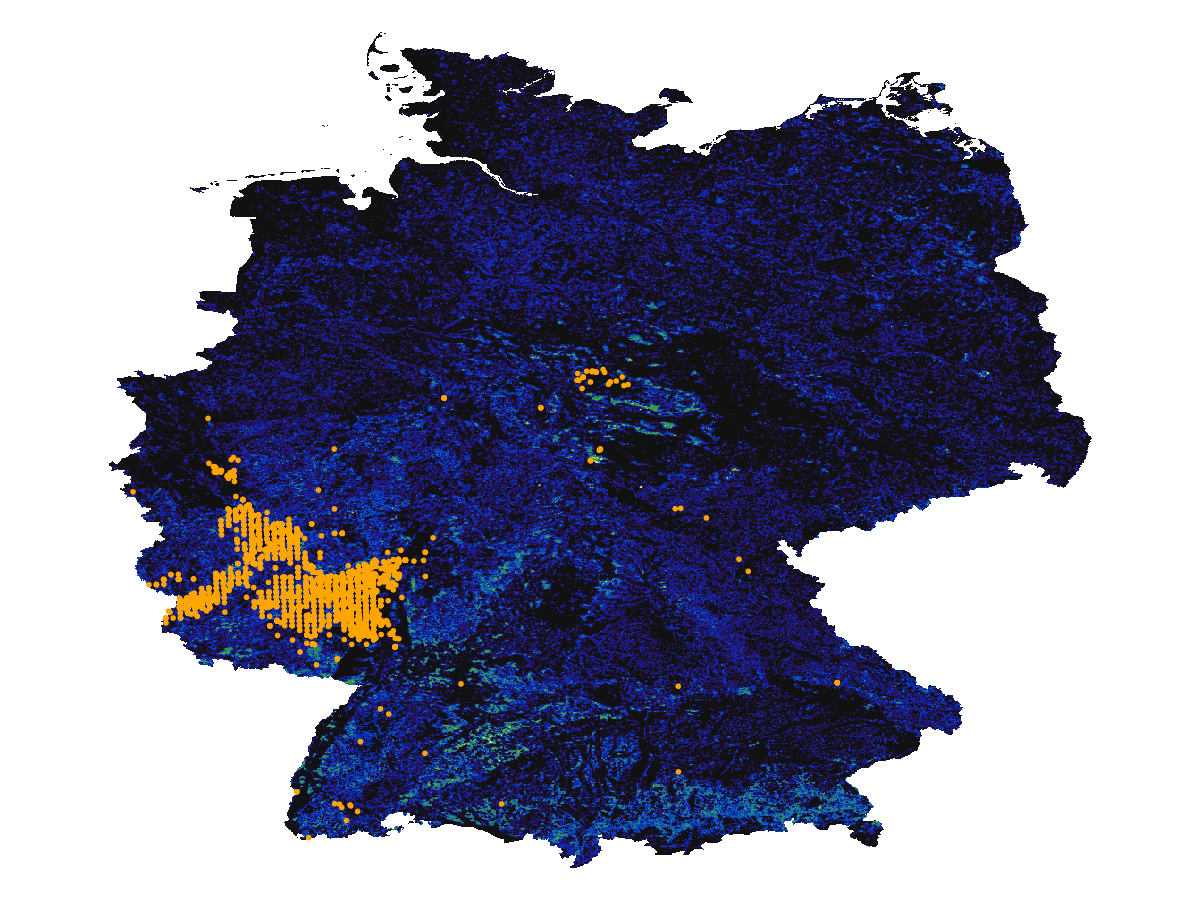
Code for the figure

f, ax, plt = heatmap(
    trim(layer);
    colormap = :linear_kbgyw_5_98_c62_n256,
    axis = (; aspect = DataAspect()),
)
scatter!(mask(presences, DEU); color = :orange, markersize = 4)
hidespines!(ax)
hidedecorations!(ax)

A note about vectors of occurrences

The reason why mask called on a GBIF result is not mutating the result is that GBIF results also store the query that was used. For this reason, it makes little sense to modify this object. The non-mutating mask returns a vector of GBIF records, which for most purposes can be used in-place of the result - this is because GBIF records are AbstractOccurrence, and vectors of these are handled correctly by the package.