Building the BIOCLIM model

In this tutorial, we will build the BIOCLIM model of species distribution, using only basic functions from SpeciesDistributionToolkit.

using SpeciesDistributionToolkit
using CairoMakie

The BIOCLIM model

The SDeMo package comes with an implementation of the BIOCLIM model that is much easier to use, and can actually be tuned to make predictions. This tutorial is meant to explore different operations on layers.

Getting the data

We will get data on the occurrences of the New-Zealand long-tailed bat from GBIF, and then use data from CHELSA to estimate the climatic envelope of this species.

species = taxon("Chalinolobus tuberculatus"; strict = false)
query = [
    "occurrenceStatus" => "PRESENT",
    "hasCoordinate" => true,
    "country" => "NZ",
    "limit" => 300,
]
presences = occurrences(species, query...)
while length(presences) < count(presences)
    occurrences!(presences)
end

This species is endemic to New Zealand (and we limited the occurrences to this country anyway), so we can use the occurrence information to define a bounding box. Because the output of a GBIF queries uses the occurrences interface, we can simply get the latitude and longitude of each occurrence:

occ = filter(!ismissing, place(presences))
left, right = extrema(first.(occ))
bottom, top = extrema(last.(occ))
bbox = (; bottom, top, left, right)

(bottom = -46.993808, top = -35.280772, left = 167.53, right = 176.71114)

We will get our environmental variables from CHELSA1:

dataprovider = RasterData(CHELSA1, BioClim)

RasterData{CHELSA1, BioClim}(CHELSA1, BioClim)

The two layers we use to build this model are annual mean temperature and annual total precipitation:

temp = SDMLayer(dataprovider; layer = 1, bbox...)
prec = SDMLayer(dataprovider; layer = 12, bbox...)

SDM Layer with 372229 Int16 cells
	Proj string: +proj=longlat +datum=WGS84 +no_defs
	Grid size: (1407, 1103)

The BIOCLIM model

The BIOCLIM model is an envelope model in which the percentile of an environmental condition in the sites where the species is found is transformed into a score. Specifically, a species at the 50th percentile has a score of 1 (the highest possible value), and a species at the 1st and 99th percentile are considered to be equivalent. In other words, species should "prefer" their median environment.

The score is calculated as

$$2\times (\frac{1}{2}-\parallel Q-\frac{1}{2}\parallel )$$

where $Q$ is the quantile for one variable at one pixel; the final score is the minimum value for each pixel across all variables.

To calculate the scores of the BIOCLIM model, we need to get the quantiles for each variable by only considering the sites where the species is present:

Qt = quantize(temp, presences)
Qp = quantize(prec, presences)

SDM Layer with 372229 Float64 cells
	Proj string: +proj=longlat +datum=WGS84 +no_defs
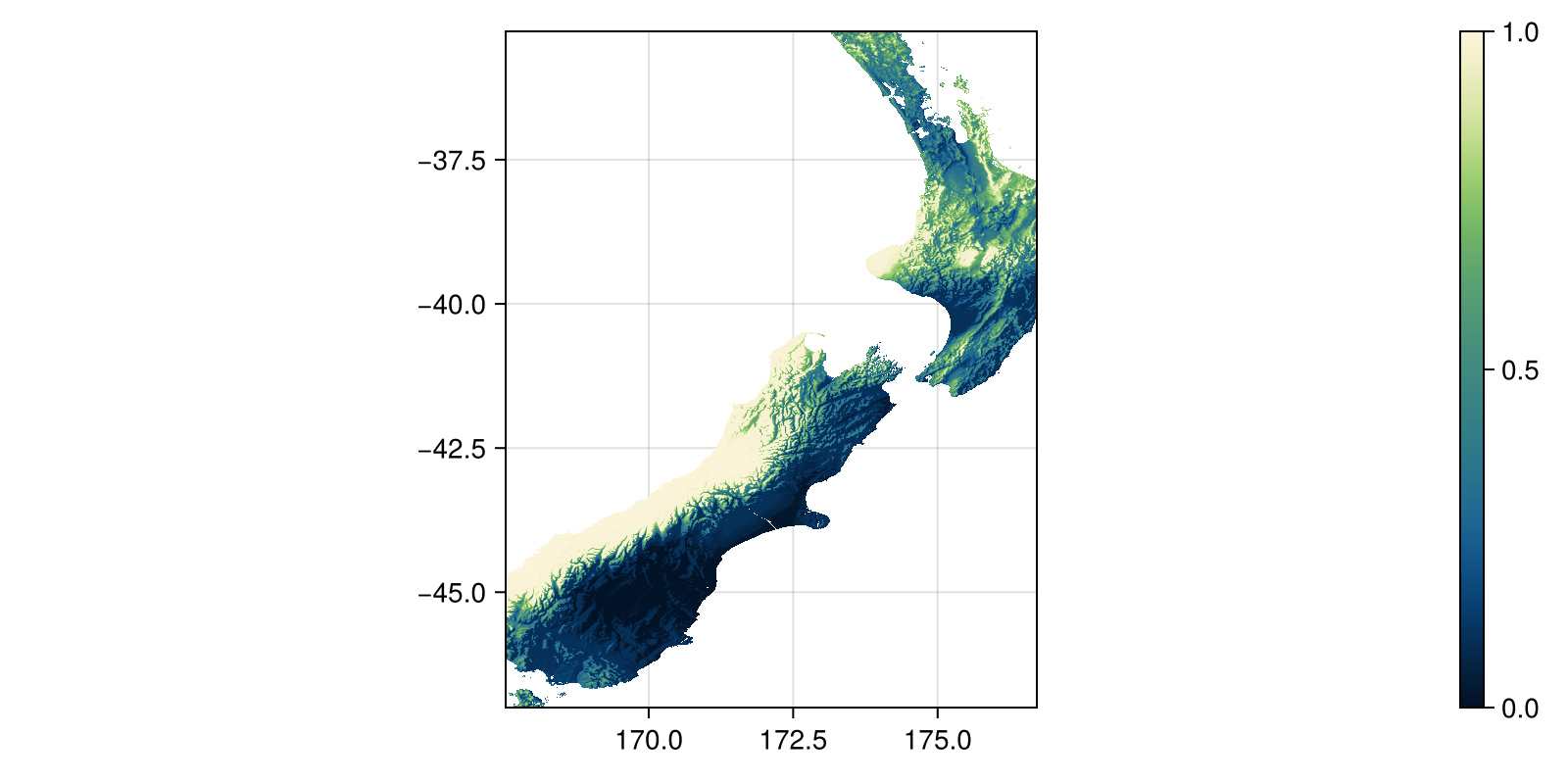
	Grid size: (1407, 1103)

We can plot the map of quantiles for precipitation:

Code for the figure

fig, ax, hm = heatmap(
    Qp;
    colormap = :navia,
    figure = (; size = (800, 400)),
    axis = (; aspect = DataAspect()),
)
Colorbar(fig[:, end + 1], hm)

In order to turn the quantiles into a score, we will be chaining together a few operations. First, the transformation of layers into layers of quantiles, then the transformation of the score, and finally the selection of the minimum value across all layers:

function BC(
    layers::Vector{<:SDMLayer},
    presences::T,
) where {T <: AbstractOccurrenceCollection}
    score = (Q) -> 2.0 .* (0.5 .- abs.(Q .- 0.5))
    Q = [quantize(layer, presences) for layer in layers]
    S = score.(Q)
    return mosaic(minimum, S)
end

BC (generic function with 1 method)

BIOCLIM selects the minimum value to reflect the fact that an organism presence is likely to be prevented in areas where one of the environmental variables are far outside the range of observations for this species.

Be careful about the occurrence status!

We have requested only presences from the GBIF API, but if we were to write a more general version of this function, it would make sense to filter the records with an occurrence status of "absent".

Making predictions

We can now call this function to get the score at each pixel:

bc = BC([temp, prec], presences)

SDM Layer with 372229 Float64 cells
	Proj string: +proj=longlat +datum=WGS84 +no_defs
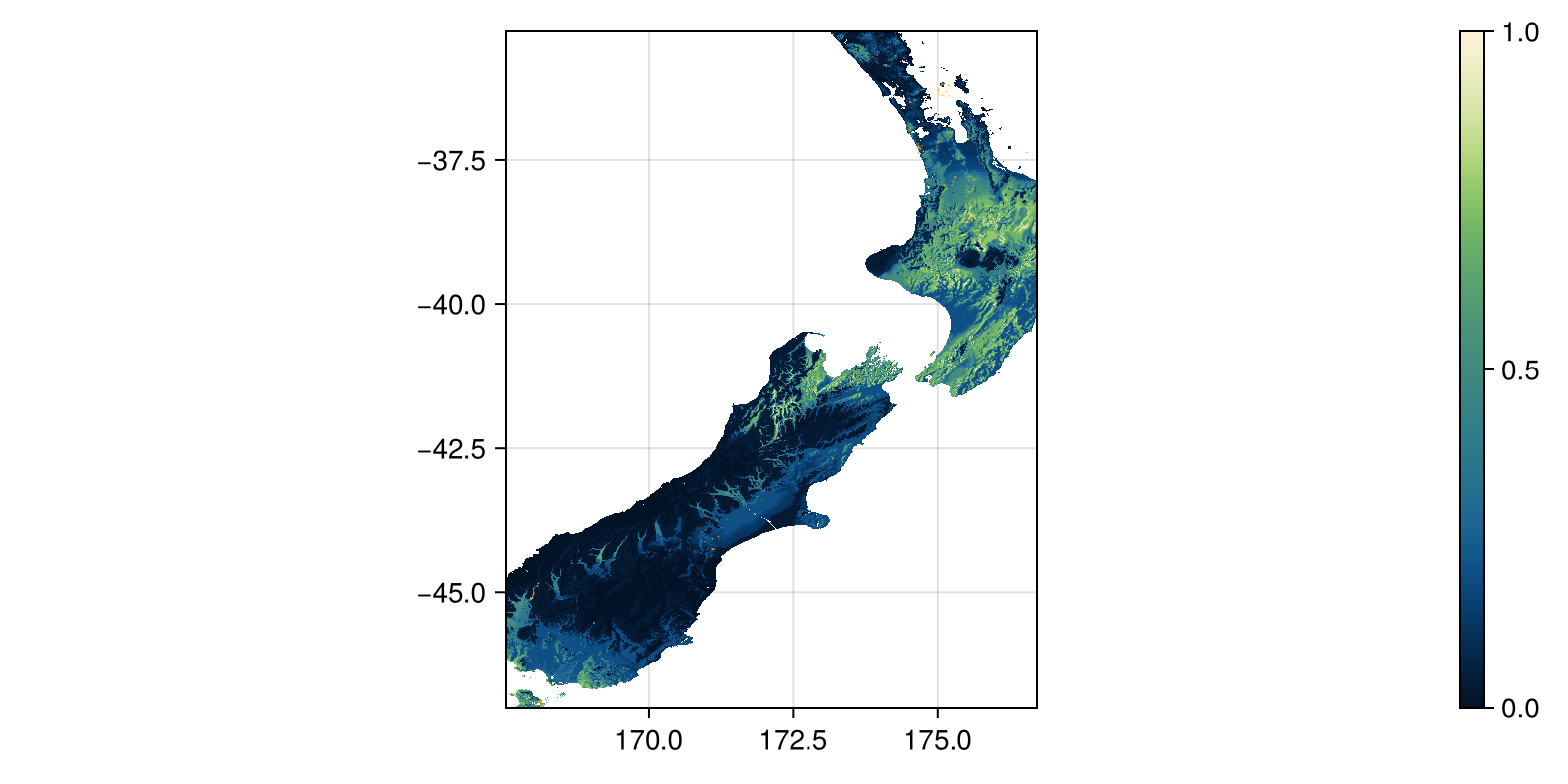
	Grid size: (1407, 1103)

The interpretation of this score is, essentially, the most restrictive environmental condition found at this specific place. We can map this, and also superimpose the presence data:

Code for the figure

fig, ax, hm = heatmap(
    bc;
    colormap = :navia,
    figure = (; size = (800, 400)),
    axis = (; aspect = DataAspect()),
)
scatter!(presences; color = :orange, markersize = 1, colorrange = (0, 1))
Colorbar(fig[:, end + 1], hm)