Calculating climate novelty

In this tutorial, we will download historical and projected future climate data, measure the climate novelty for each pixel, and provide a map showing this climate novelty.

using SpeciesDistributionToolkit

using Statistics
using CairoMakie

Accessing future data involves the Dates standard library, to make an explicit reference to years in the dataset.

import Dates

Accessing historical climate data

In order to only load a reasonable amount of data, we will specify a bounding box for the area we are interested in:

spatial_extent = (left = 23.42, bottom = 34.75, right = 26.41, top = 35.74)

(left = 23.42, bottom = 34.75, right = 26.41, top = 35.74)

Note that the bounding box is given in WGS84. Although layers can use any projection, we follow the GeoJSON specification and use WGS84 for point data. This includes species occurrence, and all polygons.

Finding bounding boxes

The bboxfinder website is a really nice tool to rapidly draw and get the coordinates for a bounding box.

We will get the BioClim data from CHELSA v1. CHELSA v1 offers access to the 19 original bioclim variable, and their projection under a variety of CMIP5 models/scenarios. These are pretty large data, and so this operation may take a while in terms of download/read time. The first time you run this command will download the data, and the next calls will read them from disk.

dataprovider = RasterData(CHELSA1, BioClim)

RasterData{CHELSA1, BioClim}(CHELSA1, BioClim)

We can search the layer that correspond to annual precipitation and annual mean temperature in the list of provided layers:

layers_code = findall(
    v -> contains(v, "Annual Mean Temperature") | contains(v, "Annual Precipitation"),
    layerdescriptions(dataprovider),
)

2-element Vector{String}:
 "BIO12"
 "BIO1"

The first step is quite simply to grab the reference state for the annual precipitation, by specifying the layer and the spatial extent:

historical = [SDMLayer(dataprovider; layer = l, spatial_extent...) for l in layers_code];

Although we specificed a bounding box, the entire layer has been downloaded, so if we want to use it in another area, it will simply be read from the disk, which will be much faster.

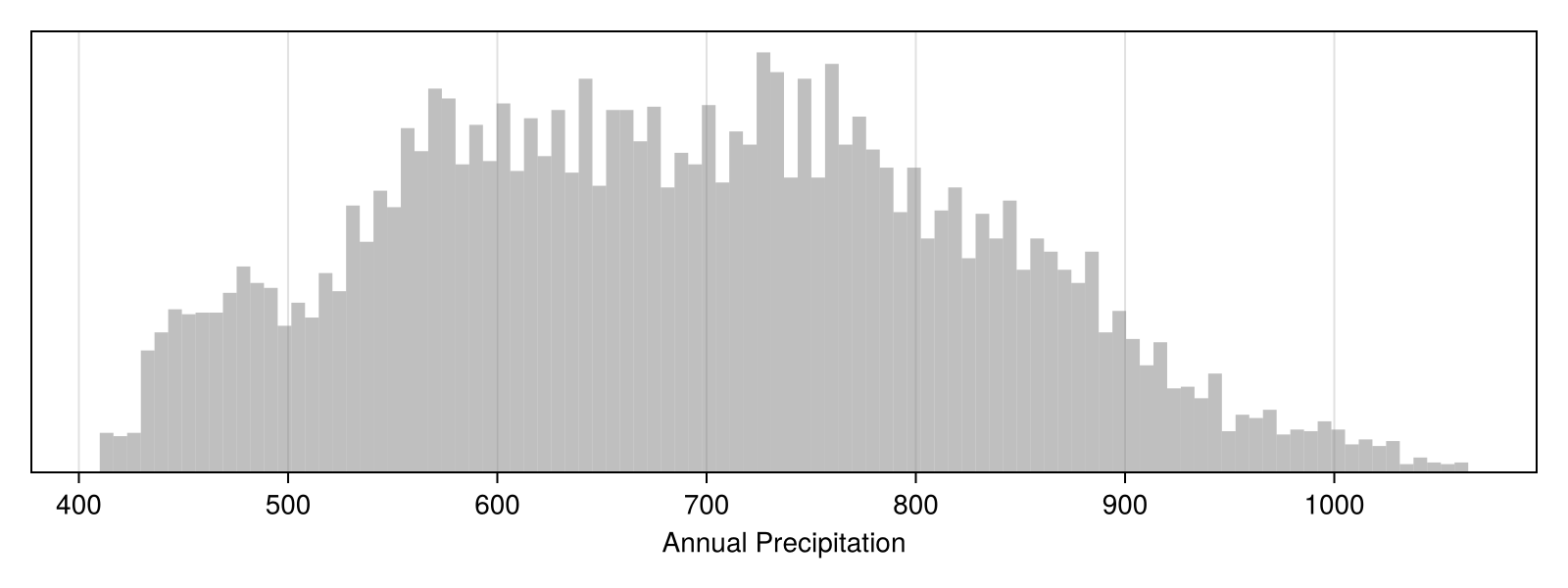
We can have a little look at this dataset by checking the density of the values for the first layer (we can pass a layer to a Makie function directly):

Code for the figure

f, ax, plt = hist(
    historical[1]; color = (:grey, 0.5),
    figure = (; size = (800, 300)),
    axis = (; xlabel = layerdescriptions(dataprovider)[layers_code[1]]),
    bins = 100,
)
ylims!(ax; low = 0)
hideydecorations!(ax)

Accessing future climate data

In the next step, we will download the projected climate data under RCP85. This requires setting up a projection object, which is composed of a scenario and a model. This information is used by the package to verify that this combination exists within the dataset we are working with.

projection = Projection(RCP85, IPSL_CM5A_MR)

Projection{RCP85, IPSL_CM5A_MR}(RCP85, IPSL_CM5A_MR)

Future data are available for different years, so we will take a look at what years are available:

available_timeperiods = SimpleSDMDatasets.timespans(dataprovider, projection)

2-element Vector{Pair{Year, Year}}:
 Year(2041) => Year(2060)
 Year(2061) => Year(2080)

Available scenarios and models

This website has a full description of each dataset, accessible from the top-level menu, which will list the scenarios, layers, models, etc., for each dataset.

If we do not specify an argument, the data retrieved will be the ones for the closest timespan. Getting the projected temperature is the same call as before, except we now pass an additional argument – the projection.

projected = [
    SDMLayer(
        dataprovider,
        projection; 
        layer = l,
        spatial_extent...,
        timespan = last(available_timeperiods),
    ) for l in layers_code
];

Re-scaling the variables

In order to compare the variables, we will first re-scale them so that they have mean zero and unit variance. More accurately, because we want to compare the historical and projected data, we will use the mean and standard deviation of the historical data as the baseline:

μ = mean.(historical)
σ = std.(historical)

2-element Vector{Float64}:
 135.6347881772658
  26.893110881710868

cr_historical = (historical .- μ) ./ σ;

cr_projected = (projected .- μ) ./ σ;

Note that these operations are applied to historical and projected, which are both vectors of layers. This is because we can broadcast operations on layers as if they were regular Julia arrays.

Measuring climate novelty

We will use a simple measure of climate novelty, which is defined as the smallest Euclidean distance between a cell in the raster and all the possible cells in the future raster.

To have a way to store the results, we will start by making a copy of one of the input rasters:

Δclim = similar(cr_historical[1])

SDM Layer with 12834 Float64 cells
	Proj string: +proj=longlat +datum=WGS84 +no_defs
	Grid size: (119, 360)

And then, we can loop over the positions to find the minimum distance. To speed up the calculation, we will store the values of the projected layers in their own objects first:

vals = values.(cr_projected)

for position in keys(cr_historical[1])
    dtemp = (cr_historical[1][position] .- vals[1]) .^ 2.0
    dprec = (cr_historical[2][position] .- vals[2]) .^ 2.0
    Δclim[position] = minimum(sqrt.(dtemp .+ dprec))
end

Because we have stored the information about the smallest possible distance directly inside the raster, we can plot it. Large values on this map indicate that this area will experience more novel climatic conditions under the scenario/model we have specified.

Code for the figure

fig, ax, hm = heatmap(
    Δclim;
    colormap = :lipari,
    figure = (; size = (800, 400)),
    axis = (; aspect = DataAspect()),
)
Colorbar(fig[:, end + 1], hm)