Generate fauxcurrences
using SpeciesDistributionToolkit
import Random
using CairoMakie
Getting observed occurrence data
Get the observation data in the correct format, which is an array of matrices with two rows (longitude, latitude) and one column for observed occurrence. This is usually an array of observations that are a subtype of AbstractOccurenceCollection (data returned from the GBIF package work), but all that matters is that this is a matrix with longitudes in the first row, and latitudes in the second row. The matrix has to be column-major, with observations as columns. To make sure that we cover a reasonable spatial extent, we will look at the rather small area in space (part of the Gaspésie region):
bbox = (bottom = 43.28, left = -66.5, top = 47.20, right = -59.45)
layer = SDMLayer(RasterData(CHELSA1, BioClim); layer = 1, bbox...)
SDM Layer with 159491 Int16 cells
Proj string: +proj=longlat +datum=WGS84 +no_defs
Grid size: (472, 847)We will pick three species of Iris that are found in this area:
taxa = taxon.(["Iris hookeri", "Iris versicolor", "Iris pseudacorus"])
observations = [
    occurrences(t,
        layer,
        "occurrenceStatus" => "PRESENT",
        "limit" => 300) for t in taxa
]
3-element Vector{GBIFRecords}:
GBIF records: downloaded 144 out of 144
GBIF records: downloaded 300 out of 1245
GBIF records: downloaded 95 out of 95The last step is to turn these occurrences into a matrix of latitudes and longitudes:
obs = [Fauxcurrences.get_valid_coordinates(o, layer) for o in observations];The observed data are distributed this way:
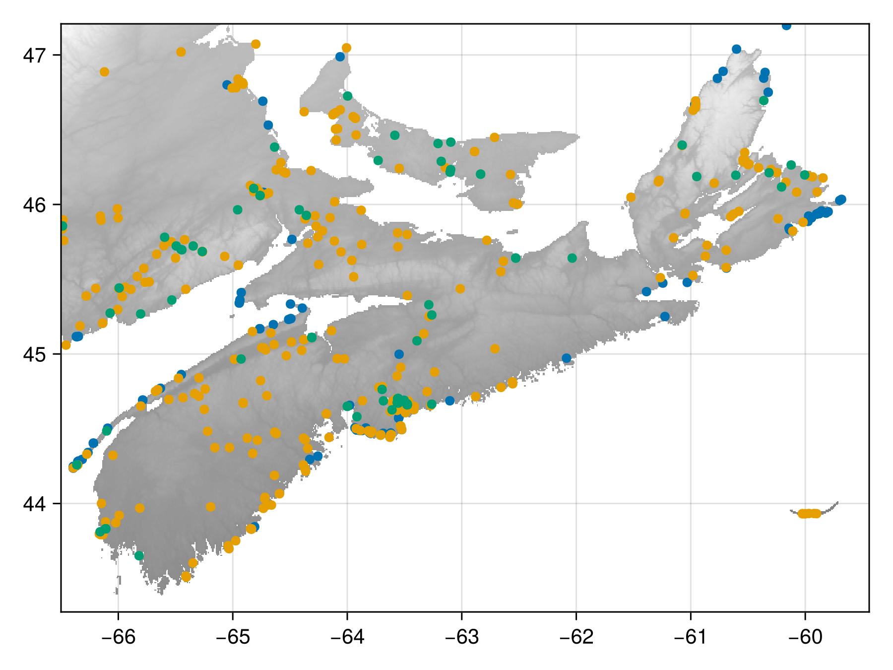
Code for the figure
heatmap(layer; colormap = [:white, :gray])
for i in eachindex(taxa)
    scatter!(obs[i]; label = taxa[i].name)
end
Preparing the run
We need to decide on the number of points (pseudo-occurrences) to generate, and the weight matrix. The number of points to generate is, by default, the number of observations in the original dataset, but this can be changed to generate balanced samples. Here, we will pick 80 as a target number of occurrences:
points_to_generate = fill(50, length(obs))3-element Vector{Int64}:
50
50
50The weight matrix is used to determine whether intra or inter-specific distances are more important in the distribution score. For example, this will set up a scoring scheme where intra-specific distances count for 75% of the total. The only constraint is that the matrix W must sum to 1, which is enforced by the code internally:
W = Fauxcurrences.weighted_components(length(obs), 0.75)3×3 Matrix{Float64}:
0.25 0.0833333 0.0833333
0.0 0.25 0.0833333
0.0 0.0 0.25We then pre-allocate the objects. This is an important part of the run, as Fauxcurrences is built to not allocate more memory than needed. As such, these objects are going to be re-written many, many times. The upside is that, if this steps fits in your memory, the entire workflow will also fit in your memory.
obs_intra, obs_inter, sim_intra, sim_inter =
    Fauxcurrences.preallocate_distance_matrices(obs; samples = points_to_generate);
The entire workflow is designed to use multiple species (as most relevant questions will require multiple species). Using a single-species approach only required to pass [obs] as opposed to obs.
The next step is to measure the intra and inter-specific distances. This is an important step as all generated points will maintain the upper bounds of these distances matrices, even if the inter-specific distance are weightless.
Fauxcurrences.measure_intraspecific_distances!(obs_intra, obs);
Fauxcurrences.measure_interspecific_distances!(obs_inter, obs);
Bootstrapping an initial proposal
When the intra/inter specific distances are known, we can pre-allocate the objects to store the simulated coordinates, and then bootstrap a set of initial proposals.
sim = Fauxcurrences.preallocate_simulated_points(obs; samples = points_to_generate);
Fauxcurrences.bootstrap!(sim, layer, obs, obs_intra, obs_inter, sim_intra, sim_inter);
To prepare the scoring of the initial solution, we need to bin the distances between the actual and simulated data. Note that the package will never allow points in the simulated occurrences to create a distance matrix where the maximum distance is larger than the maximum distance in the empirical matrix.
bin_intra = [
    Fauxcurrences._bin_distribution(obs_intra[i], maximum(obs_intra[i])) for
    i in axes(obs_intra, 1)
];
bin_inter = [
    Fauxcurrences._bin_distribution(obs_inter[i], maximum(obs_inter[i])) for
    i in axes(obs_inter, 1)
];
bin_s_intra = [
    Fauxcurrences._bin_distribution(sim_intra[i], maximum(obs_intra[i])) for
    i in axes(obs_intra, 1)
];
bin_s_inter = [
    Fauxcurrences._bin_distribution(sim_inter[i], maximum(obs_inter[i])) for
    i in axes(obs_inter, 1)
];
This version of the _bin_distribution function is allocating an array for the bins, but the internal function is over-writing it, to avoid unwanted allocations. From the binned distances, we calucate the initial divergence. This will be the starting point between the observed and simulated distributions, and the score that we want to improve. Note that it accounts for the weights in the matrix. This step will return a vector, the sum of which is the total divergence between the matrices.
D = Fauxcurrences.score_distributions(W, bin_intra, bin_s_intra, bin_inter, bin_s_inter)
sum(D)
0.27766494052371093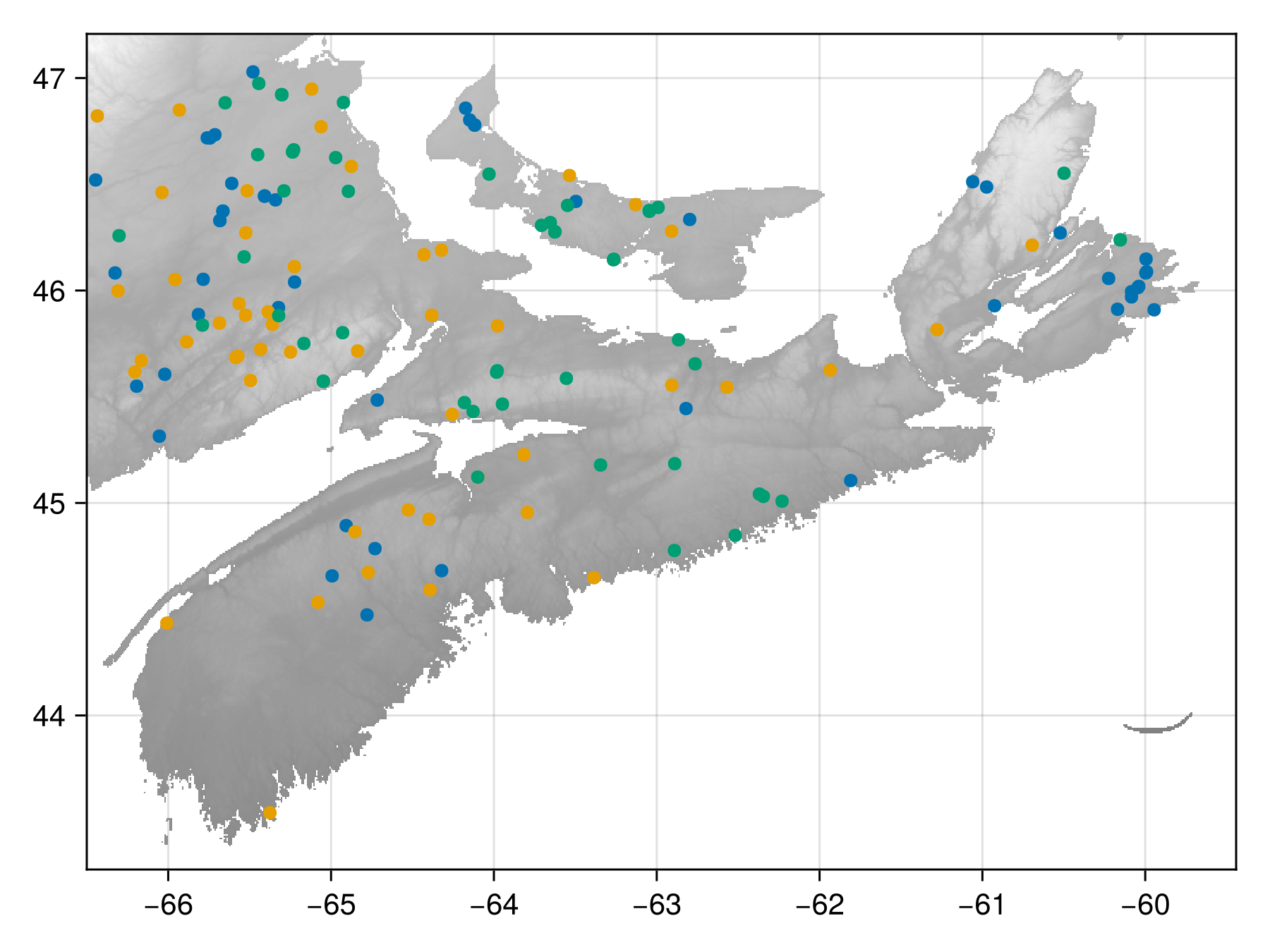
Code for the figure
heatmap(layer; colormap = [:white, :gray])
for i in eachindex(taxa)
    scatter!(sim[i]; label = taxa[i].name)
end
Generating the fauxcurrences
We can now setup the actual run. This step has infinitely many variations, as Fauxcurrences only offers a method to perform a single step forward. In most cases, using e.g. ProgressMeter will be a good way to track the progress of the run, and to allow, for example, to stop it when a collection of criteria (absolute/relative divergence, globally, on average, or per-species) are met. For the sake of simplicity, we return the sum of all divergences, measures for 500000 timesteps.
progress = zeros(Float64, 500_000)
progress[1] = sum(D)0.27766494052371093The step! function takes most of what we have allocated so far, which is a lot, but allows considerable performance gains. The last argument to step! is the current divergence, and the return value of step! (in addition to modifying the simulated points) is the new divergence.
Before running the actual loop, it is a good idea to time a handful of steps.
Why a handful? Because Julia do be compiling, and because depending on the structure of your points, the problem might be more or less difficult to solve. In practice, using ProgressMeter will make the timing of the whole process a lot more informative. In this simple version, we rely on a manually created progress report. Note that we stop the process when we have done at least 1×10⁵ steps, with no improvement over the last 2×10³.
for i in axes(progress, 1)[2:end]
    progress[i] = Fauxcurrences.step!(
        sim,
        layer,
        W,
        obs_intra,
        obs_inter,
        sim_intra,
        sim_inter,
        bin_intra,
        bin_inter,
        bin_s_intra,
        bin_s_inter,
        progress[i - 1],
    )
    if i > 100_000
        if abs(progress[i] - progress[i - 2000]) <= 1e-5
            break
        end
    end
    if iszero(i % 10_000)
        println(
            "[$(lpad(round(Int64, 100*(i/length(progress))), 3))%]\tJS-divergence: $(round(progress[i]; digits=3))",
        )
    end
end
[ 2%] JS-divergence: 0.118
[ 4%] JS-divergence: 0.104
[ 6%] JS-divergence: 0.097
[ 8%] JS-divergence: 0.096
[ 10%] JS-divergence: 0.096
[ 12%] JS-divergence: 0.091
[ 14%] JS-divergence: 0.091
[ 16%] JS-divergence: 0.091
[ 18%] JS-divergence: 0.089
[ 20%] JS-divergence: 0.089The call to step! is... lengthy. The reason for this is very simple: step! will update as much information as it can in place when a change is made. This means that there are no objects created (only changed). The downside is that the function needs to be given a lot of information.
Depending on the number of species (and the structure of the weight matrix), this step will be taking a little while. This is because, assuming we want n points for r species, each step has a complexity on the order of rn², which isn't terribly good.
Analyzing the fauxcurrences
When the run is done, it would makes sense to look at the total improvement (or to plot the timeseries of the improvement):
final_progress =
    round(progress[begin] / progress[findlast(x -> x > 0, progress)]; digits = 3)
println(
    "Improvement: $(final_progress) ×",
)
Improvement: 3.135 ×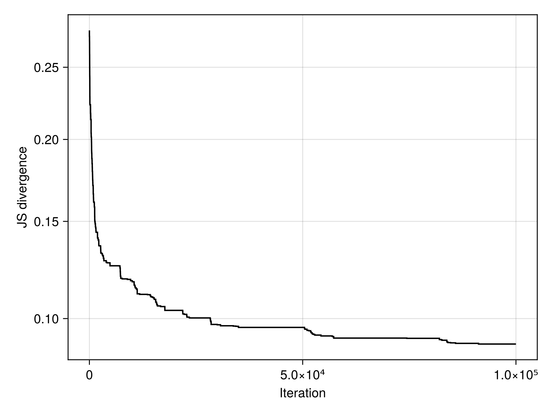
Code for the figure
lines(
    progress[1:findlast(x -> x > 0, progress)];
    axis = (; yscale = sqrt, xlabel = "Iteration", ylabel = "JS divergence"),
    color = :black,
)
Note that for a small number of iterations (like we used here), this improvement is unlikely to be very large; note also that the returns (in terms of improvement over time) are very much diminishing. The good news is that re-starting the process is as easy as running the loop with calls to step! again, as the package has modified the matrices, and is ready to restart at any time. This is useful for checkpointing.
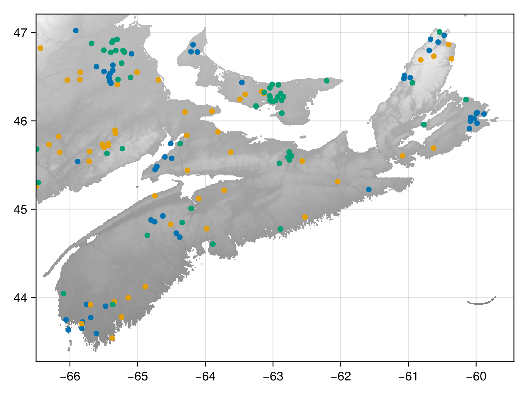
The final disposition of the fauxcurrences is:
Code for the figure
heatmap(layer; colormap = [:white, :gray])
for i in eachindex(taxa)
    scatter!(sim[i]; label = taxa[i].name)
end
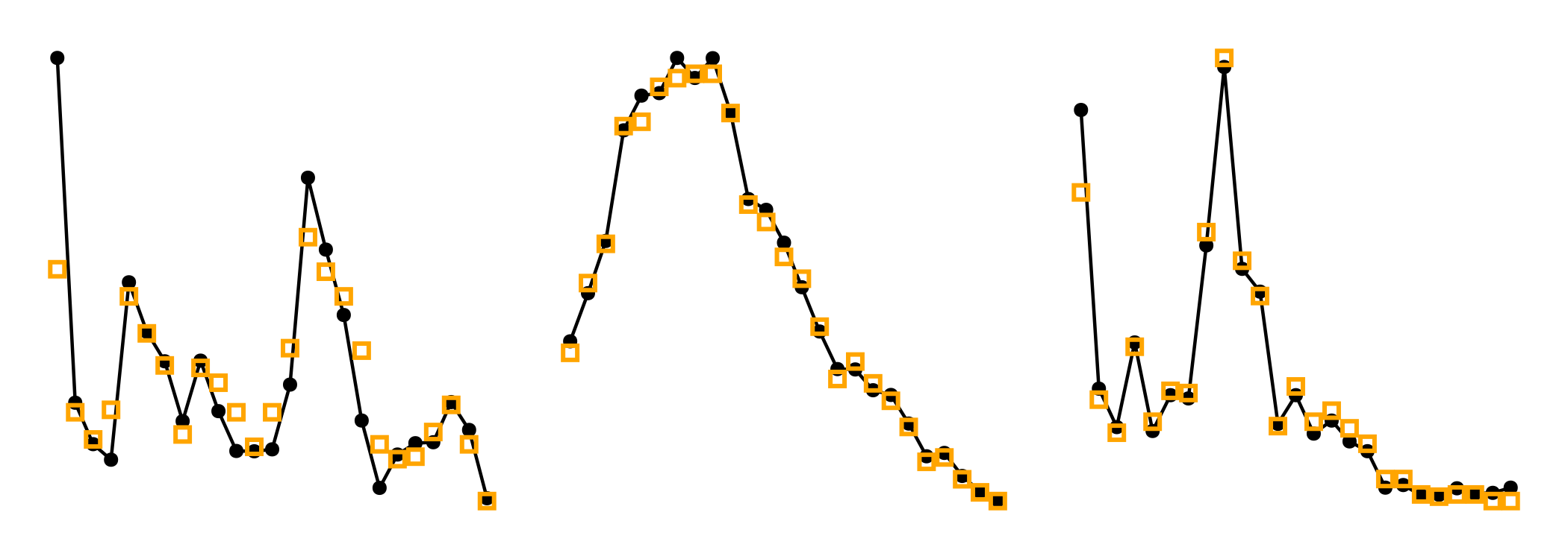
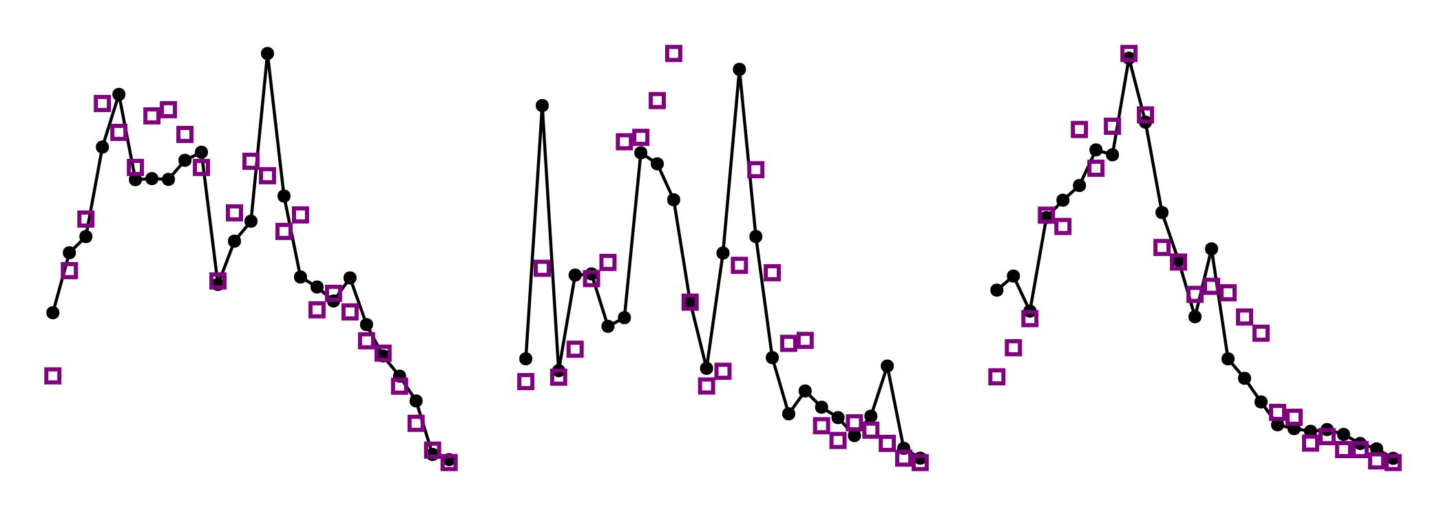
We can also look at the per-matrix score, out of all the distance bins (set as a package-wide variable, Fauxcurrences._number_of_bins, which you are encouraged to tweak) – under a good fit, the lines in bin_intra and bin_s_intra would overlap (same with ..._inter).
For the intra-specific distances, with observations in black and the simulation in orange, this looks like:
Code for the figure
f = Figure(; size = (700, 250))
ax1 = Axis(f[1, 1])
scatterlines!(ax1, bin_intra[1]; color = :black)
scatter!(
    ax1,
    bin_s_intra[1];
    color = :transparent,
    strokewidth = 2,
    strokecolor = :orange,
    markersize = 10,
    marker = :rect,
)
ax2 = Axis(f[1, 2])
scatterlines!(ax2, bin_intra[2]; color = :black)
scatter!(
    ax2,
    bin_s_intra[2];
    color = :transparent,
    strokewidth = 2,
    strokecolor = :orange,
    markersize = 10,
    marker = :rect,
)
ax3 = Axis(f[1, 3])
scatterlines!(ax3, bin_intra[3]; color = :black)
scatter!(
    ax3,
    bin_s_intra[3];
    color = :transparent,
    strokewidth = 2,
    strokecolor = :orange,
    markersize = 10,
    marker = :rect,
)
[hidespines!(ax) for ax in [ax1, ax2, ax3]]
[hidedecorations!(ax) for ax in [ax1, ax2, ax3]]
For the components of the inter-specific distance matrix, this gives the following plot:
Code for the figure
f = Figure(; size = (700, 250))
ax1 = Axis(f[1, 1])
scatterlines!(ax1, bin_inter[1]; color = :black)
scatter!(
    ax1,
    bin_s_inter[1];
    color = :transparent,
    strokewidth = 2,
    strokecolor = :purple,
    markersize = 10,
    marker = :rect,
)
ax2 = Axis(f[1, 2])
scatterlines!(ax2, bin_inter[2]; color = :black)
scatter!(
    ax2,
    bin_s_inter[2];
    color = :transparent,
    strokewidth = 2,
    strokecolor = :purple,
    markersize = 10,
    marker = :rect,
)
ax3 = Axis(f[1, 3])
scatterlines!(ax3, bin_inter[3]; color = :black)
scatter!(
    ax3,
    bin_s_inter[3];
    color = :transparent,
    strokewidth = 2,
    strokecolor = :purple,
    markersize = 10,
    marker = :rect,
)
[hidespines!(ax) for ax in [ax1, ax2, ax3]]
[hidedecorations!(ax) for ax in [ax1, ax2, ax3]]
Note that the inter-specific distances are not fully respected, but this is because we decided to give more weight to the intra-specific distances in the initial parameters.