Training SDMs with SDeMo

The purpose of this vignette is to take a whistle-stop tour of the what the package has to offer. We will see how to train a model, cross-validate it, select variables, tune hyper-parameters, use bootstraping to measure uncertainty, show partial response curves, calculate varialble importances through bootstraping and Shapley values, and generate counterfactual inputs.

Mapping the outputs

The functions to interact with raster data, and present the outputs of models as maps, are implemented as part of SpeciesDistributionToolkit (SDT). There is a follow-up tutorial that focuses on visualisation of SDM outputs.

This vignette is very terse and is not an introduction to using or interpreting these models!

Setting up the environment

using SpeciesDistributionToolkit
using Statistics
using CairoMakie
using PrettyTables

The package comes with a series of demonstration data, that represent the presences and absences of Sitta whiteheadi at about 1500 locations in Corsica, with 19 bioclim environmental variables:

X, y = SDeMo.__demodata()
size(X)

(19, 1484)

Setting up the model

We will start with an initial model that uses a PCA to transform the data, and then a Naive Bayes Classifier for the classification. Note that this is the partial syntax where we use the default threshold, and all the variables:

sdm = SDM(MultivariateTransform{PCA}, NaiveBayes, X, y)

PCATransform → NaiveBayes → P(x) ≥ 0.5

Transformations

The transformations will by default only account for the presences. This is motivated by the fact that absences will often be pseudo-absences, and therefore should not be used to transform the data. There are ways to use absences to transform the data as well, which are presented in the SDeMo manual.

Initial cross-validation

Throughout this demonstration, we will use the same splits between validation and training data, with 10 folds:

folds = kfold(sdm; k = 10);

Using the same splits is important because it will provide a fair basis of comparison for the different models.

Before starting any manipulation, we can start cross-validating the model: this will return a named tuple with the confusion matrices for validation and training data:

cv = crossvalidate(sdm, folds);

The reason why we return the confusion matrices as opposed to directly measuring statistics is that we have more freedom to manipulate the data, without needing to re-run the analysis. For example, we can get the average of a handful of measures on this first step of cross validation:

measures = [mcc, balancedaccuracy, ppv, npv, trueskill, markedness]
cvresult = [measure(set) for measure in measures, set in cv]
pretty_table(
    hcat(string.(measures), cvresult);
    alignment = [:l, :c, :c],
    backend = Val(:markdown),
    header = ["Measure", "Validation", "Training"],
    formatters = ft_printf("%5.3f", [2, 3]),
)

Measure	Validation	Training
mcc	0.501	0.502
balancedaccuracy	0.749	0.748
ppv	0.730	0.730
npv	0.776	0.776
trueskill	0.498	0.497
markedness	0.506	0.506

By default, calling a function to measure model performance (the full list is in the manual) on a series of confusion matrices will return the average. Adding the true argument returns a tuple with the 95% CI:

mcc(cv.validation, true)

(0.5014894802983206, 0.04048032968194452)

If we want to get a simple idea of what the MCC is for the validation data for all folds, we can use:

mcc.(cv.validation)

10-element Vector{Float64}:
 0.411601475294833
 0.5674044484888594
 0.4655712348560116
 0.47520253719491684
 0.4012480832119629
 0.5132755881718536
 0.5282350793547591
 0.4949922840967364
 0.6023685038544081
 0.5549955684588657

The associated confidence interval is

ci(cv.validation, mcc)

0.04048032968194452

Note that cross-validation does not train the model. This is meant to convey the idea that cross-validation is letting us know whether the model is good enough to be trained. If we want to forgo variable selection, we can train the model with

train!(sdm)

PCATransform → NaiveBayes → P(x) ≥ 0.39

Variable selection

We will now select variables using forward selection, but with the added constraint that the first variable (annual mean temperature) must be included:

forwardselection!(sdm, folds, [1])

PCATransform → NaiveBayes → P(x) ≥ 0.322

This operation will retrain the model. We can now look at the list of selected variables:

variables(sdm)

6-element Vector{Int64}:
  1
  3
  6
  4
 15
  2

Is this making a difference in terms of cross-validation?

cv2 = crossvalidate(sdm, folds)
measures = [mcc, balancedaccuracy, ppv, npv, trueskill, markedness]
cvresult = [measure(set) for measure in measures, set in cv2]
pretty_table(
    hcat(string.(measures), cvresult);
    alignment = [:l, :c, :c],
    backend = Val(:markdown),
    header = ["Measure", "Validation", "Training"],
    formatters = ft_printf("%5.3f", [2, 3]),
)

Measure	Validation	Training
mcc	0.788	0.785
balancedaccuracy	0.898	0.896
ppv	0.842	0.842
npv	0.938	0.937
trueskill	0.796	0.792
markedness	0.780	0.779

Quite clearly! Before thinking about the relative importance of variables, we will take a look at the thresold.

Moving threshold classification

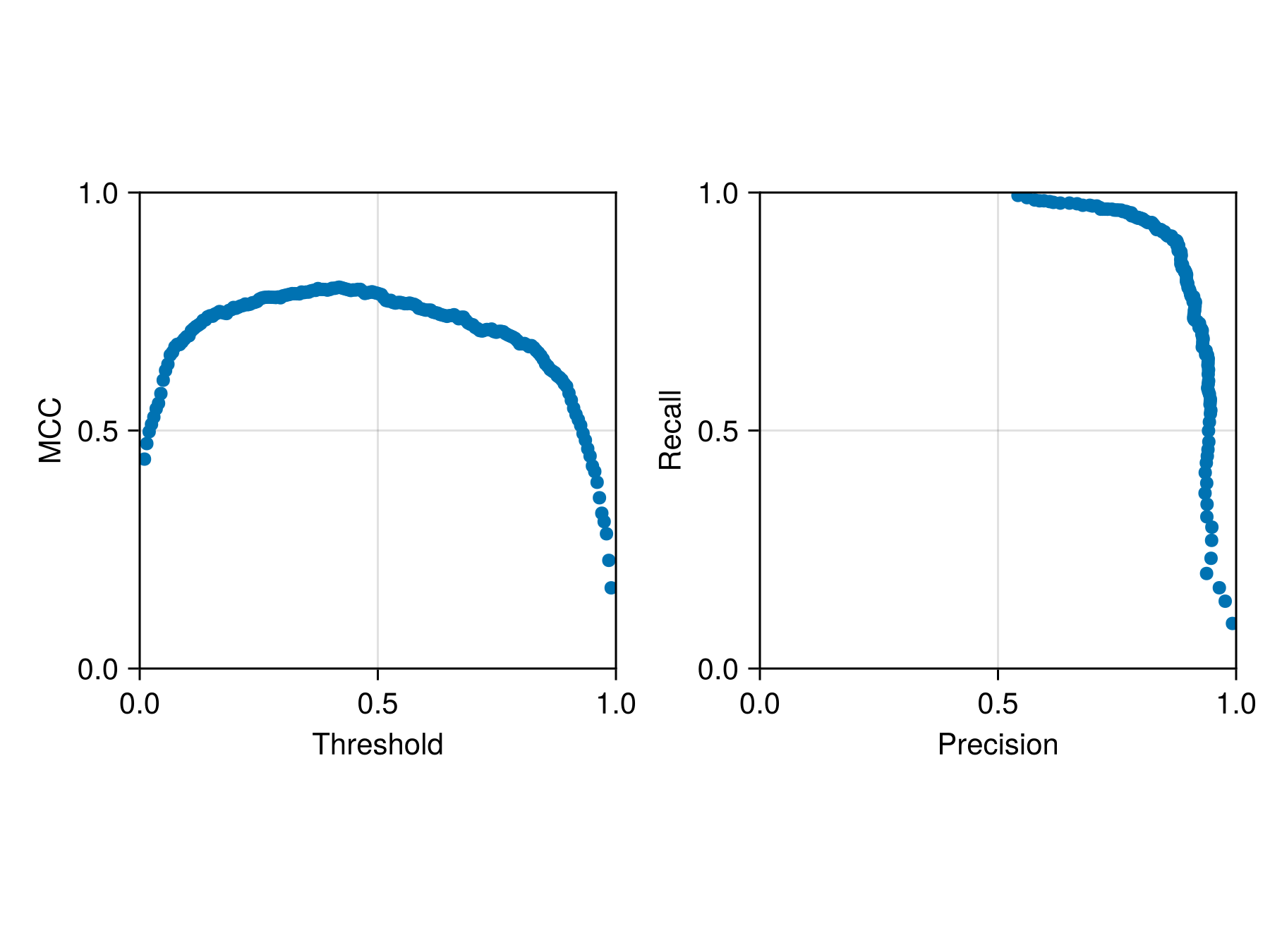
The crossvalidate function comes with an optional argument to specify the threshold between a positive and negative outcome. We can use this to figure out the best possible threshold:

thresholds = LinRange(0.01, 0.99, 200)
cv3 = [crossvalidate(sdm, folds; thr = t) for t in thresholds];

We can plot the simplified version of this analysis (averaged across all folds for each value of the threshold):

Code for the figure

f = Figure()
ax = Axis(f[1, 1]; aspect = 1, xlabel = "Threshold", ylabel = "MCC")
scatter!(ax, thresholds, [mean(mcc.(s.validation)) for s in cv3])
ax2 = Axis(f[1, 2]; aspect = 1, xlabel = "Precision", ylabel = "Recall")
scatter!(
    ax2,
    [mean(SDeMo.precision.(s.validation)) for s in cv3],
    [mean(SDeMo.recall.(s.validation)) for s in cv3],
)
xlims!(ax, 0.0, 1.0)
ylims!(ax, 0.0, 1.0)
xlims!(ax2, 0.0, 1.0)
ylims!(ax2, 0.0, 1.0)

For reference, the threshold at the end of this process is:

threshold(sdm)

0.3215740401355837

Variable importance

We can evaluate the importance of each variable by bootstrap, where the values of this variable are randomized, and the absolute value of the difference in model performance is returned (averaged across all folds):

varimp = variableimportance(sdm, folds)

6-element Vector{Float64}:
 0.27323841649892033
 0.07389908443010518
 0.28296741279358817
 0.17955314447782553
 0.03419082453433911
 0.002253220156847351

In relative terms, this is:

pretty_table(
    hcat(variables(sdm), varimp ./ sum(varimp));
    alignment = [:l, :c],
    backend = Val(:markdown),
    header = ["Variable", "Importance"],
    formatters = (ft_printf("%5.3f", 2), ft_printf("%d", 1)),
)

Variable	Importance
1	0.323
3	0.087
6	0.334
4	0.212
15	0.040
2	0.003

Partial response curve

Another way to look at the effect of variables is to use the partial response curves. For example, we can look at the predictions of the model between 5 and 15 degrees:

prx, pry = partialresponse(sdm, 1, LinRange(5.0, 15.0, 100); threshold = false);

Note that we use threshold=false to make sure that we look at the score that is returned by the classifier, and not the thresholded version.

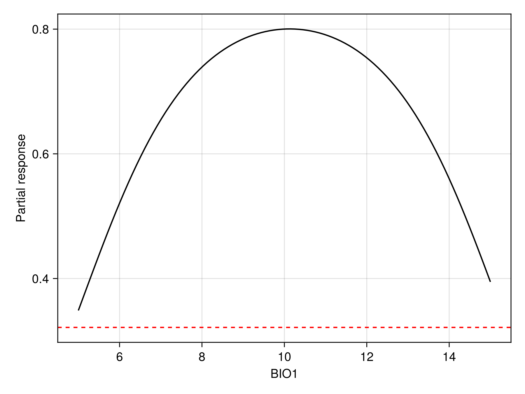
Code for the figure

f = Figure()
ax = Axis(f[1, 1]; xlabel = "BIO1", ylabel = "Partial response")
lines!(ax, prx, pry; color = :black)
hlines!(ax, [threshold(sdm)]; color = :red, linestyle = :dash)

We can also show the response surface using two variables:

prx, pry, prz = partialresponse(sdm, variables(sdm)[1:2]..., (100, 100); threshold = false);

Note that the last element returned in this case is a two-dimensional array, as it makes sense to visualize the result as a heatmap. Although the idea of a the partial response curves generalizes to more than two dimensions, it is not supported by the package.

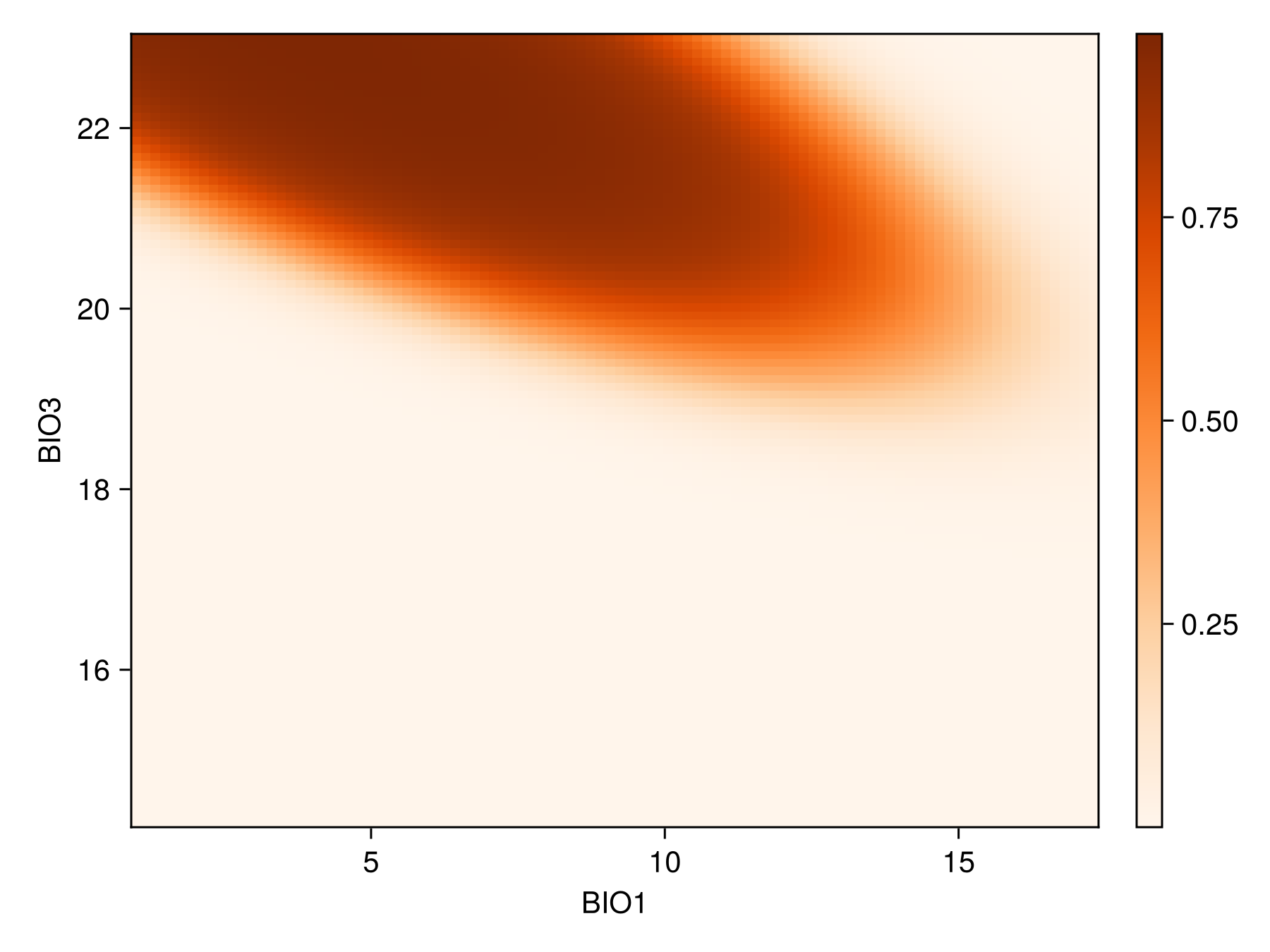
Code for the figure

f = Figure()
ax = Axis(f[1, 1]; xlabel = "BIO$(variables(sdm)[1])", ylabel = "BIO$(variables(sdm)[2])")
cm = heatmap!(prx, pry, prz; colormap = :Oranges)
Colorbar(f[1, 2], cm)

Inflated partial responses

Inflated partial responses replace the average value by other values drawn from different quantiles of the variables:

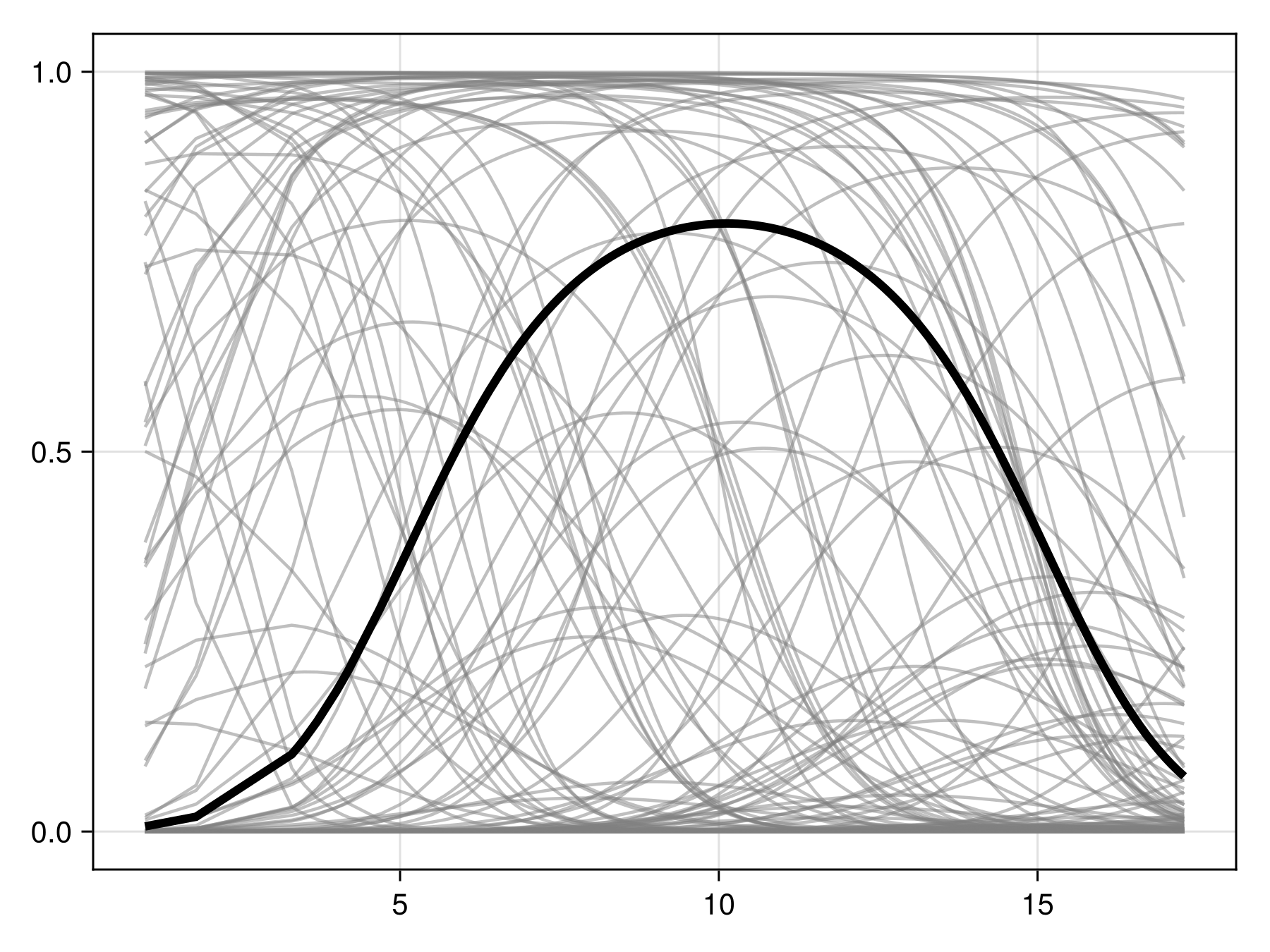
Code for the figure

f = Figure()
ax = Axis(f[1, 1])
prx, pry = partialresponse(sdm, 1; inflated = false, threshold = false)
for i in 1:200
    ix, iy = partialresponse(sdm, 1; inflated = true, threshold = false)
    lines!(ax, ix, iy; color = (:grey, 0.5))
end
lines!(ax, prx, pry; color = :black, linewidth = 4)

Measuring uncertainty with bagging

We can wrap our model into an homogeneous ensemble:

ensemble = Bagging(sdm, 20)
train!(ensemble)

{PCATransform → NaiveBayes → P(x) ≥ 0.322} × 20

Ensemble models can be used in the same way as regular models, but take an extra keyword consensus to indicate how the results from each model should be reconciled. By default, this is the median, but for uncertainty, iqr is a great choice. Note that we use threshold=false because we want to look at the distribution of the score, not the boolean output:

uncert = predict(ensemble; consensus = iqr, threshold = false);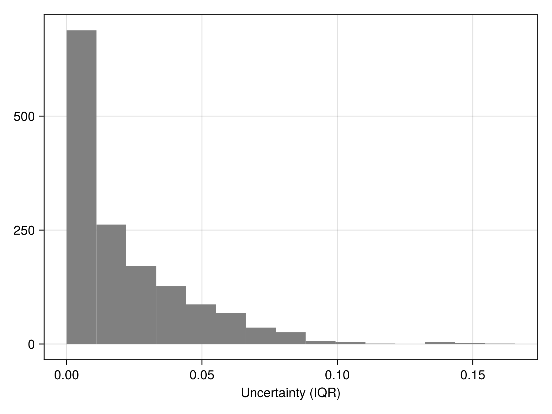

Code for the figure

hist(uncert; color = :grey, axis = (; xlabel = "Uncertainty (IQR)"))

Heterogeneous ensembles

We can setup an heterogeneous ensemble model by passing several SDMs to Ensemble:

m1 = SDM(MultivariateTransform{PCA}, NaiveBayes, X, y)
m2 = SDM(RawData, BIOCLIM, X, y)
m3 = SDM(MultivariateTransform{PCA}, BIOCLIM, X, y)
variables!(m2, [1, 12])
hm = Ensemble(m1, m2, m3)

An ensemble model with:
	 PCATransform → NaiveBayes → P(x) ≥ 0.5
	 RawData → BIOCLIM → P(x) ≥ 0.01
	 PCATransform → BIOCLIM → P(x) ≥ 0.01

We can train this model in the same way:

train!(hm)

An ensemble model with:
	 PCATransform → NaiveBayes → P(x) ≥ 0.39
	 RawData → BIOCLIM → P(x) ≥ 0.11
	 PCATransform → BIOCLIM → P(x) ≥ 0.102

And get predictions:

predict(hm; consensus = median, threshold = false)[1:10]

10-element Vector{Float64}:
 0.5181674565560821
 0.5023696682464455
 0.39178515007898895
 0.6350710900473934
 0.20853080568720372
 0.639106860018156
 0.05055292259083721
 0.2559241706161137
 0.18957345971563977
 0.593996840442338

Note that the ensemble models (Bagging and Ensemble) are supported by the explain, partialresponse, and counterfactual functions.

Explaining predictions

We can perform the (MCMC version of) Shapley values measurement, using the explain method:

[explain(sdm, v; observation = 3) for v in variables(sdm)]

6-element Vector{Float64}:
 -0.19
  0.04
 -0.18
 -0.005
  0.02
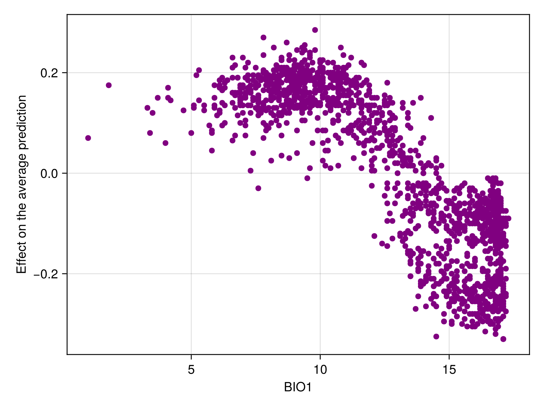
 -0.005

These values are returned as the effect of this variable's value on the average prediction for this observation.

We can also produce a figure that looks like the partial response curve, by showing the effect on a variable on each training instance:

Code for the figure

f = Figure()
ax = Axis(f[1, 1]; xlabel = "BIO1", ylabel = "Effect on the average prediction")
scatter!(ax, features(sdm, 1), explain(sdm, 1; threshold = true); color = :purple)

Counterfactuals

In the final example, we will focus on generating a counterfactual input, i.e. a set of hypothetical inputs that lead the model to predicting the other outcome. Internally, candidate points are generated using the Nelder-Mead algorithm, which works well enough but is not compatible with categorical data.

We will pick one prediction to flip:

inst = 4

4

And look at its outcome:

outcome = predict(sdm)[inst]

true

Our target is expressed in terms of the score we want the counterfactual to reach (and not in terms of true/false, this is very important):

target = outcome ? 0.9threshold(sdm) : 1.1threshold(sdm)

0.28941663612202534

The actual counterfactual is generated as:

cf = counterfactual(
    sdm,
    instance(sdm, inst; strict = false),
    target,
    200.0;
    threshold = false,
)

19-element Vector{Float64}:
  13.228503368671777
   3.812552349998173
  20.8990908875656
 505.0859650219775
  16.7
  -0.31810197778322247
  18.3
   5.6000000000000005
  13.200000000000001
  14.299999999999997
   0.30000000000000004
 924.0
 135.0
  14.0
  47.974493367547375
 382.0
  61.0
  72.0
 283.0

The last value (set to 200.0 here) is the learning rate, which usually needs to be tuned. The countefactual input for the observation we are interested in is:

pretty_table(
    hcat(variables(sdm), instance(sdm, inst), cf[variables(sdm)]);
    alignment = [:l, :c, :c],
    backend = Val(:markdown),
    header = ["Variable", "Obs.", "Counterf."],
    formatters = (ft_printf("%4.1f", [2, 3]), ft_printf("%d", 1)),
)

Variable	Obs.	Counterf.
1	6.6	13.2
3	21.0	20.9
6	-1.6	-0.3
4	505.1	505.1
15	48.0	48.0
2	3.8	3.8

We can check the prediction that would be made on the counterfactual:

predict(sdm, cf)

false

Conclusion

This vignette offered a very quick overview of what the SDeMo package does. The integration with the rest of the SpeciesDistributionToolkit ecosystem is detailed in the main documentation.