Use with the SDeMo package

In this tutorial, we will reproduce (the spirit of) the excellent tutorial on SDMs by Damaris Zurell, using the same species and location, a similar dataset, but a slightly different algorithm.

using SpeciesDistributionToolkit
using CairoMakie
using Statistics
using Dates

Note that this tutorial is not showing all the capacities of the SDeMo package!

Getting the data

CHE = SpeciesDistributionToolkit.gadm("CHE");

In order to simplify the code, we will start from a list of bioclim variables that have been picked to optimize the model:

bio_vars = [1, 11, 5, 8, 6]

5-element Vector{Int64}:
  1
 11
  5
  8
  6

We get the data on these variables from CHELSA2:

provider = RasterData(CHELSA2, BioClim)
layers = [
    SDMLayer(
        provider;
        layer = x,
        left = 0.0,
        right = 20.0,
        bottom = 35.0,
        top = 55.0,
    ) for x in bio_vars
];

And we then clip and trim to the polygon describing Switzerland:

layers = [trim(mask!(layer, CHE)) for layer in layers];
layers = map(l -> convert(SDMLayer{Float32}, l), layers);

The next step is to get the data, using the eBird dataset:

ouzel = taxon("Turdus torquatus")
presences = occurrences(
    ouzel,
    first(layers),
    "occurrenceStatus" => "PRESENT",
    "limit" => 300,
    "datasetKey" => "4fa7b334-ce0d-4e88-aaae-2e0c138d049e",
)
while length(presences) < count(presences)
    occurrences!(presences)
end

And after this, we prepare a layer with absences. Note that this code is not particularly beautiful but will be fixed when we release the occurrences interface package as part of a next version.

presencelayer = zeros(first(layers), Bool)
for occ in mask(presences, CHE)
    presencelayer[occ.longitude, occ.latitude] = true
end

The next step is to generate a pseudo-absence mask. We will sample based on the distance to an observation, by also preventing pseudo-absences to be less than 4km from an observation:

background = pseudoabsencemask(DistanceToEvent, presencelayer)
bgpoints = backgroundpoints(nodata(background, d -> d < 4), 2sum(presencelayer))

SDM Layer with 45336 Bool cells
	Proj string: +proj=longlat +datum=WGS84 +no_defs
	Grid size: (239, 543)

We can take a minute to visualize the dataset, as well as the location of presences and pseudo-absences:

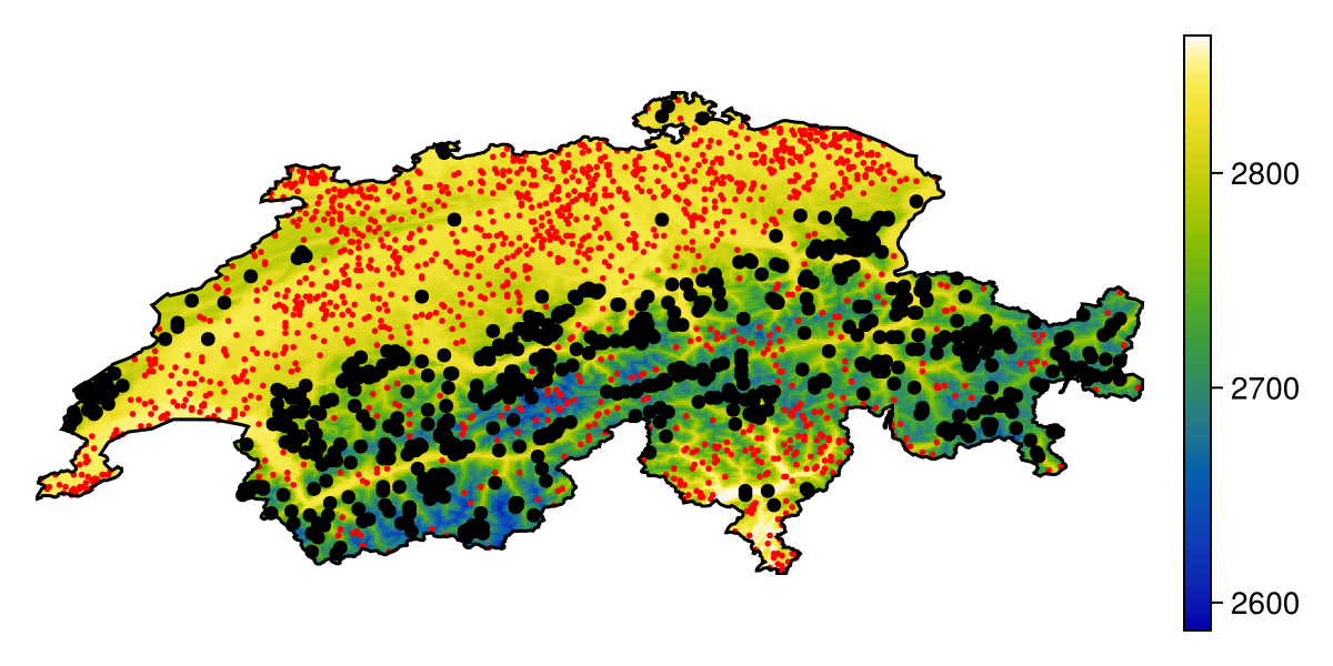
Code for the figure

f = Figure(; size = (600, 300))
ax = Axis(f[1, 1]; aspect = DataAspect())
hm = heatmap!(ax,
    first(layers);
    colormap = :linear_bgyw_20_98_c66_n256,
)
scatter!(ax, presencelayer; color = :black)
scatter!(ax, bgpoints; color = :red, markersize = 4)
lines!(ax, CHE.geometry[1]; color = :black)
Colorbar(f[1, 2], hm)
hidedecorations!(ax)
hidespines!(ax)

Setting up the model

These steps are documented as part of the SDeMo documentation. The only difference here is that rather than passing a matrix of features and a vector of labels, we give a vector of layers (features), and the two layers for presences and absences:

sdm = SDM(MultivariateTransform{PCA}, DecisionTree, layers, presencelayer, bgpoints)

PCATransform → DecisionTree → P(x) ≥ 0.5

We use a decision tree classifier, which SDeMo provides (admittedly in a rough version) out of the box.

Out of curiosity, we can check the expected performance of the model:

folds = kfold(sdm);
cv = crossvalidate(sdm, folds; threshold = true);
mean(mcc.(cv.validation))

0.6946615976540111

We will now train the model on all the training data.

train!(sdm)

PCATransform → DecisionTree → P(x) ≥ 0.176

Making the first prediction

We can predict using the model by giving a vector of layers as an input. This will return the output as a layer as well:

prd = predict(sdm, layers; threshold = false)

SDM Layer with 69967 Float64 cells
	Proj string: +proj=longlat +datum=WGS84 +no_defs
	Grid size: (239, 543)

Decision trees, in oredr to avoid overfitting, are pretty small – indeed, the default version in SDeMo is capped at 12 nodes, with a maximal depth of 7. This is because there is no limit to how much decision trees can overfit. But as a result, the map representing these predictions can look a little coarse:

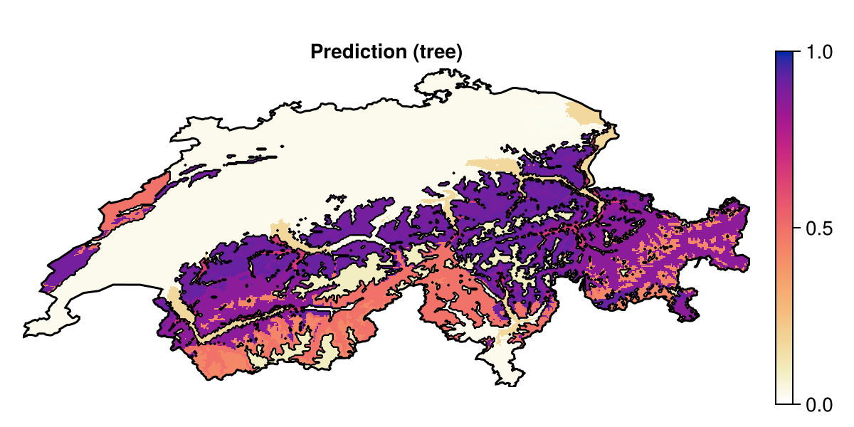
Code for the figure

f = Figure(; size = (600, 300))
ax = Axis(f[1, 1]; aspect = DataAspect(), title = "Prediction (tree)")
hm = heatmap!(ax, prd; colormap = :linear_worb_100_25_c53_n256, colorrange = (0, 1))
contour!(ax, predict(sdm, layers); color = :black, linewidth = 0.5)
Colorbar(f[1, 2], hm)
lines!(ax, CHE.geometry[1]; color = :black)
hidedecorations!(ax)
hidespines!(ax)

In order to maintain a good predictive power with less overfitting risk, but with a finer outcome, we will rely on bagging.

ensemble = Bagging(sdm, 30)

{PCATransform → DecisionTree → P(x) ≥ 0.176} × 30

In order to further ensure that the models are learning from different parts of the dataset, we can also bootstrap which variables are accessible to each model:

bagfeatures!(ensemble)

{PCATransform → DecisionTree → P(x) ≥ 0.176} × 30

By default, the bagfeatures! function called on an ensemble will sample the variables forom the model, so that each model in the ensemble has the square root (rounded up) of the number of original variables.

About this ensemble model

The model we have constructed here is essentially a random forest. Note that the PCA is applied to each tree, so it is accounting for the selection of features.

We can now train our ensemble model – for an ensemble, this will go through each model, and retrain them with the correct input data/features.

train!(ensemble)

{PCATransform → DecisionTree → P(x) ≥ 0.176} × 30

Let's have a look at the out-of-bag performance using MCC, to make sure that there is no grievous loss of performance:

outofbag(ensemble) |> mcc

0.7077304781042998

Because this ensemble is a collection of model, we set the method to summarize all the scores as the median:

prd = predict(ensemble, layers; consensus = median, threshold = false)

SDM Layer with 69967 Float64 cells
	Proj string: +proj=longlat +datum=WGS84 +no_defs
	Grid size: (239, 543)

When the model is trained, we can make a prediction asking to report the inter-quartile range of the predictions of all models, as a measure of uncertainty:

unc = predict(ensemble, layers; consensus = iqr, threshold = false)

SDM Layer with 69967 Float64 cells
	Proj string: +proj=longlat +datum=WGS84 +no_defs
	Grid size: (239, 543)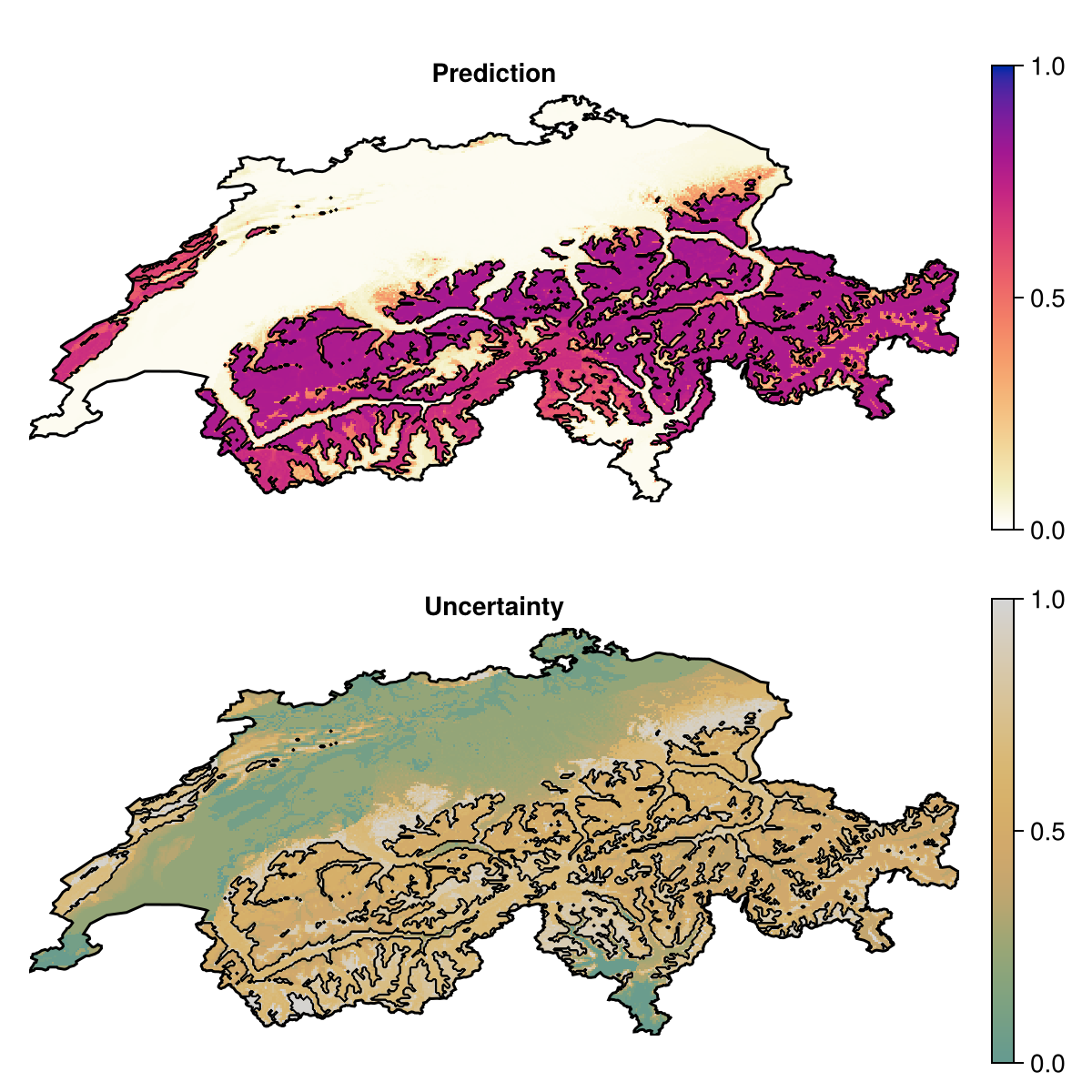

Code for the figure

f = Figure(; size = (600, 600))
ax = Axis(f[1, 1]; aspect = DataAspect(), title = "Prediction")
hm = heatmap!(ax, prd; colormap = :linear_worb_100_25_c53_n256, colorrange = (0, 1))
Colorbar(f[1, 2], hm)
contour!(
    ax,
    predict(ensemble, layers; consensus = majority);
    color = :black,
    linewidth = 0.5,
)
lines!(ax, CHE.geometry[1]; color = :black)
hidedecorations!(ax)
hidespines!(ax)
ax2 = Axis(f[2, 1]; aspect = DataAspect(), title = "Uncertainty")
hm =
    heatmap!(ax2, quantize(unc); colormap = :linear_gow_60_85_c27_n256, colorrange = (0, 1))
Colorbar(f[2, 2], hm)
contour!(
    ax2,
    predict(ensemble, layers; consensus = majority);
    color = :black,
    linewidth = 0.5,
)
lines!(ax2, CHE.geometry[1]; color = :black)
hidedecorations!(ax2)
hidespines!(ax2)

Partial responses and explanations

Like predictions, asking for a partial response or a Shapley value with a vector of layers will return the output as layers, with the value calculated for each pixel:

part_v1 = partialresponse(ensemble, layers, first(variables(sdm)); threshold = false);
shap_v1 = explain(ensemble, layers, first(variables(sdm)); threshold = false, samples = 50);

We can confirm that these two approaches broadly agree about where the effect of the first variable (temperature) is leading the model to predict presences.

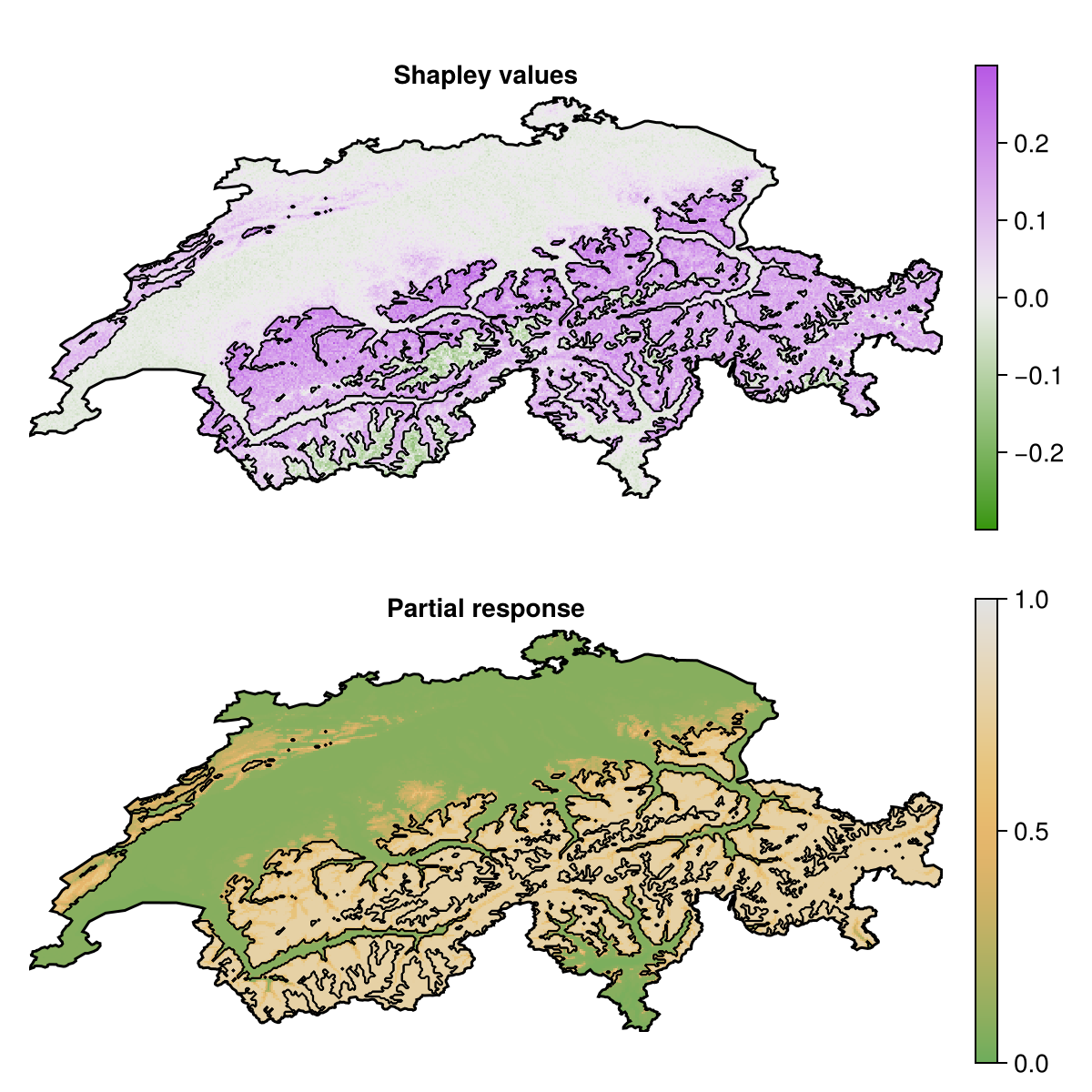
Code for the figure

f = Figure(; size = (600, 600))
ax = Axis(f[1, 1]; aspect = DataAspect(), title = "Shapley values")
hm = heatmap!(
    ax,
    shap_v1;
    colormap = :diverging_gwv_55_95_c39_n256,
    colorrange = (-0.3, 0.3),
)
contour!(
    ax,
    predict(ensemble, layers; consensus = majority);
    color = :black,
    linewidth = 0.5,
)
hidedecorations!(ax)
hidespines!(ax)
Colorbar(f[1, 2], hm)
ax2 = Axis(f[2, 1]; aspect = DataAspect(), title = "Partial response")
hm = heatmap!(ax2, part_v1; colormap = :linear_gow_65_90_c35_n256, colorrange = (0, 1))
contour!(
    ax2,
    predict(ensemble, layers; consensus = majority);
    color = :black,
    linewidth = 0.5,
)
lines!(ax2, CHE.geometry[1]; color = :black)
Colorbar(f[2, 2], hm)
hidedecorations!(ax2)
hidespines!(ax2)

We can also get the Shapley values for all layers, which will return a vector of layers, one for each included variable:

S = explain(sdm, layers; threshold = false, samples = 100);

We can then put this object into the mosaic function to get the index of which variable is the most important for each pixel:

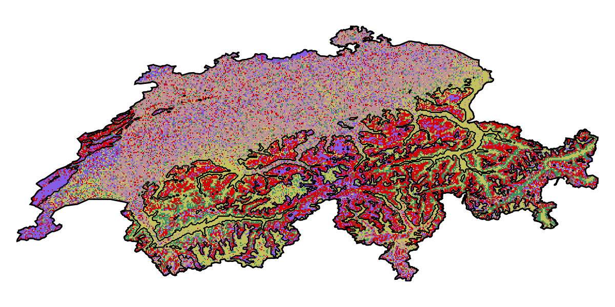
Code for the figure

f = Figure(; size = (600, 300))
ax = Axis(f[1, 1]; aspect = DataAspect())
heatmap!(
    ax,
    mosaic(v -> argmax(abs.(v)), S);
    colormap = cgrad(
        :glasbey_bw_n256,
        length(variables(sdm));
        categorical = true,
    ),
)
contour!(
    ax,
    predict(ensemble, layers; consensus = majority);
    color = :black,
    linewidth = 0.5,
)
lines!(ax, CHE.geometry[1]; color = :black)
hidedecorations!(ax)
hidespines!(ax)