Targeting Unique Climates for Sampling
This tutorial will focus on using the utilities in BiodiversityObservationNetworks.jl to use environmental data to compute rarity (how unique the environmental conditions in a location are).
It will also demonstrate how inclusion probabilities can be used to target spatially balanced samples toward rare climates, which is applicable more broadly toward targeting any specific variable of interest.
Acquiring climate data
We will use SpeciesDistributionToolkit.jl to download climate data.
using BiodiversityObservationNetworks
using SpeciesDistributionToolkit
using CairoMakie
We'll start by downloading a polygon for the state of Washington state, which is the region we will use for this tutorial.
aoi = getpolygon(PolygonData(OpenStreetMap, Places), place = "Washington State")FeatureCollection with 1 features, each with 10 propertiesWe can then load the 19 Bioclimatic variables from CHELSA as follows.
bioclim = [SDMLayer(RasterData(CHELSA1, BioClim); SpeciesDistributionToolkit.SimpleSDMPolygons.boundingbox(aoi)..., layer = i) for i in 1:19]19-element Vector{SimpleSDMLayers.SDMLayer{Int16}}:
🗺️ A 416 × 952 layer (355723 Int16 cells)
🗺️ A 416 × 952 layer (355723 Int16 cells)
🗺️ A 416 × 952 layer (355723 Int16 cells)
🗺️ A 416 × 952 layer (355723 Int16 cells)
🗺️ A 416 × 952 layer (355723 Int16 cells)
🗺️ A 416 × 952 layer (355723 Int16 cells)
🗺️ A 416 × 952 layer (355723 Int16 cells)
🗺️ A 416 × 952 layer (355723 Int16 cells)
🗺️ A 416 × 952 layer (355723 Int16 cells)
🗺️ A 416 × 952 layer (355723 Int16 cells)
🗺️ A 416 × 952 layer (355723 Int16 cells)
🗺️ A 416 × 952 layer (355723 Int16 cells)
🗺️ A 416 × 952 layer (355723 Int16 cells)
🗺️ A 416 × 952 layer (355723 Int16 cells)
🗺️ A 416 × 952 layer (355723 Int16 cells)
🗺️ A 416 × 952 layer (355723 Int16 cells)
🗺️ A 416 × 952 layer (355723 Int16 cells)
🗺️ A 416 × 952 layer (355723 Int16 cells)
🗺️ A 416 × 952 layer (355723 Int16 cells)Further documentation on the various available data can be found in SpeciesDistributionToolkit.jl's documentation.
We'll now mask the bioclimatic layers to only include regions inside Washington:
mask!(bioclim, aoi)19-element Vector{SimpleSDMLayers.SDMLayer{Int16}}:
🗺️ A 416 × 952 layer (303225 Int16 cells)
🗺️ A 416 × 952 layer (303225 Int16 cells)
🗺️ A 416 × 952 layer (303225 Int16 cells)
🗺️ A 416 × 952 layer (303225 Int16 cells)
🗺️ A 416 × 952 layer (303225 Int16 cells)
🗺️ A 416 × 952 layer (303225 Int16 cells)
🗺️ A 416 × 952 layer (303225 Int16 cells)
🗺️ A 416 × 952 layer (303225 Int16 cells)
🗺️ A 416 × 952 layer (303225 Int16 cells)
🗺️ A 416 × 952 layer (303225 Int16 cells)
🗺️ A 416 × 952 layer (303225 Int16 cells)
🗺️ A 416 × 952 layer (303225 Int16 cells)
🗺️ A 416 × 952 layer (303225 Int16 cells)
🗺️ A 416 × 952 layer (303225 Int16 cells)
🗺️ A 416 × 952 layer (303225 Int16 cells)
🗺️ A 416 × 952 layer (303225 Int16 cells)
🗺️ A 416 × 952 layer (303225 Int16 cells)
🗺️ A 416 × 952 layer (303225 Int16 cells)
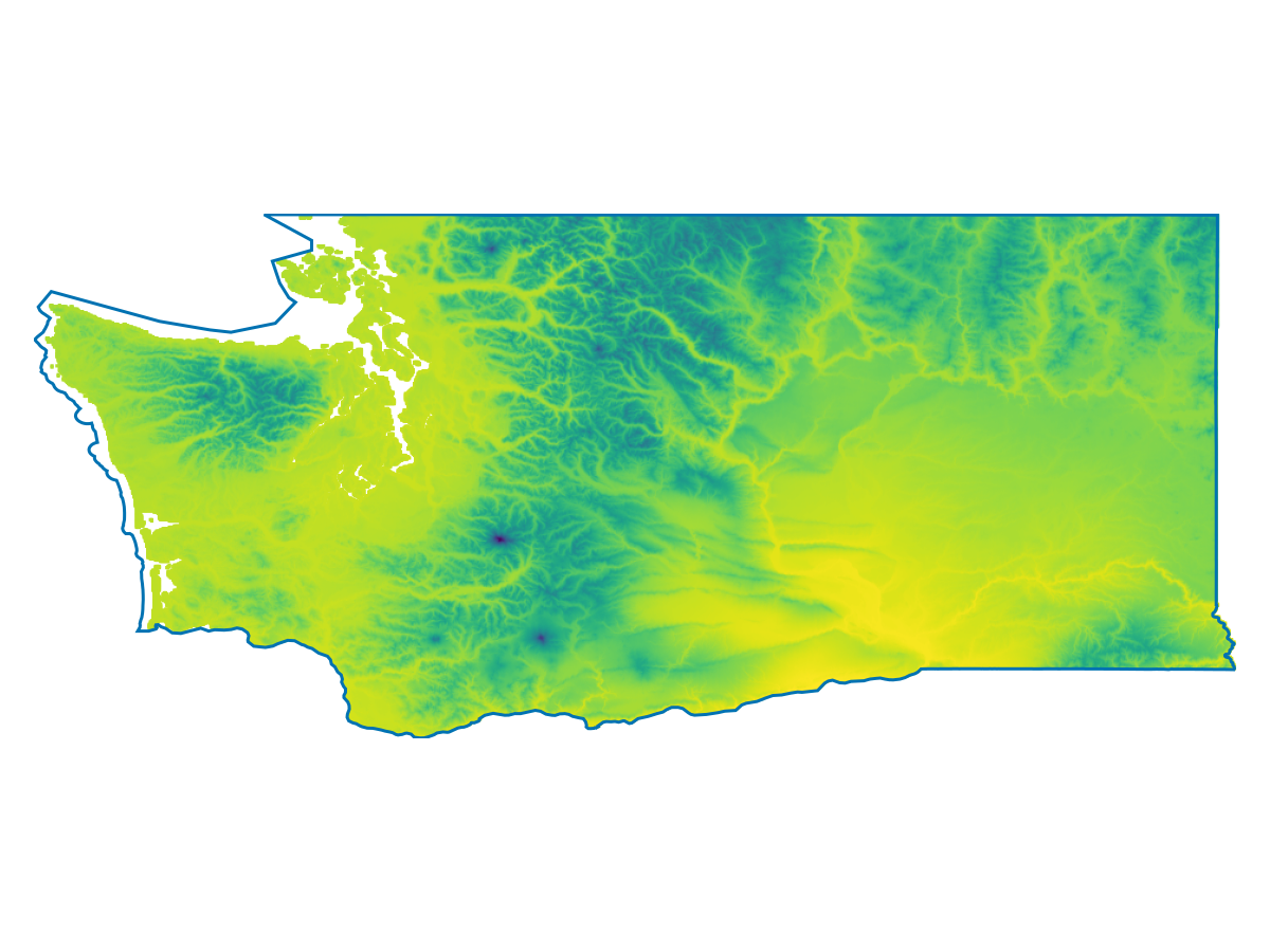
🗺️ A 416 × 952 layer (303225 Int16 cells)And now we'll visualize the first layer, which is the mean annual temperature:
Code for the figure
f = Figure()
ax = Axis(f[1,1], aspect=DataAspect())
hidedecorations!(ax)
hidespines!(ax)
heatmap!(ax, bioclim[1])
lines!(ax, aoi)
Measuring Climate Rarity
BiodiversityObservationNetworks.jl contains several utilities for quantifying how rare the environmental conditions at a particular location are.
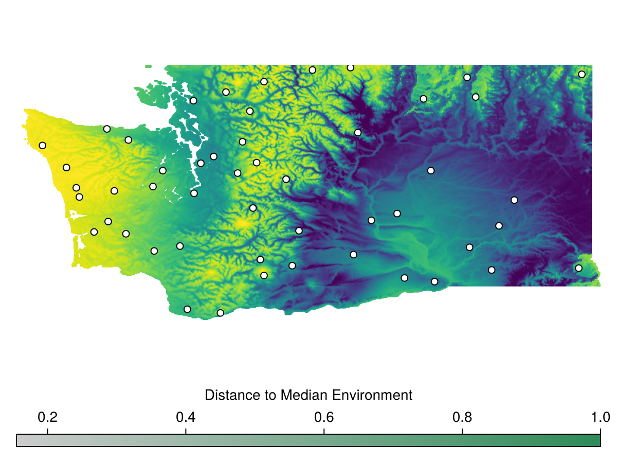
Distance to median climate
The simplest is DistanceToMedian, which is each pixel's distance in environmental space to the median environmental conditions across the domain.
All rarity, velocity, and evaluation metrics are built around the evaluate method.
The API is structured similarly to sample.
evaluate(::SamplingMetric, domain)or
evaluate(::SamplingMetric, domain, bon)for metrics that involve a BON in addition to the domain.
For DistanceToMedian, this looks like
rar = evaluate(
    DistanceToMedian(),
    bioclim
)
🗺️ A 416 × 952 layer with 303225 Float64 cells
Spatial Reference System: +proj=longlat +datum=WGS84 +no_defsWhich we can then visualize
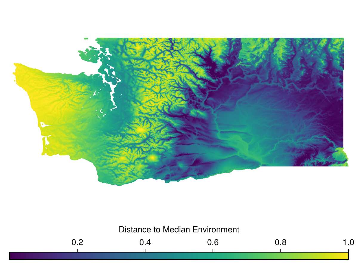
Code for the figure
f = Figure()
ax = Axis(f[1,1], aspect=DataAspect())
hidedecorations!(ax)
hidespines!(ax)
hm = heatmap!(ax, rar)
Colorbar(f[2,1], hm, vertical = false, label="Distance to Median Environment")
MultivariateEnvironmentalSimilarity
A second metric for environmental uniqueness is MultivariateEnvironmentalSimilarity, which is derived from (Mesgaran et al., 2024).
This is a similarity score, so higher values indicate similarity, lower values indicate rarity.
This can be run via
mess = evaluate(
    MultivariateEnvironmentalSimilarity(),
    bioclim
)
🗺️ A 416 × 952 layer with 303225 Float64 cells
Spatial Reference System: +proj=longlat +datum=WGS84 +no_defsand visualized
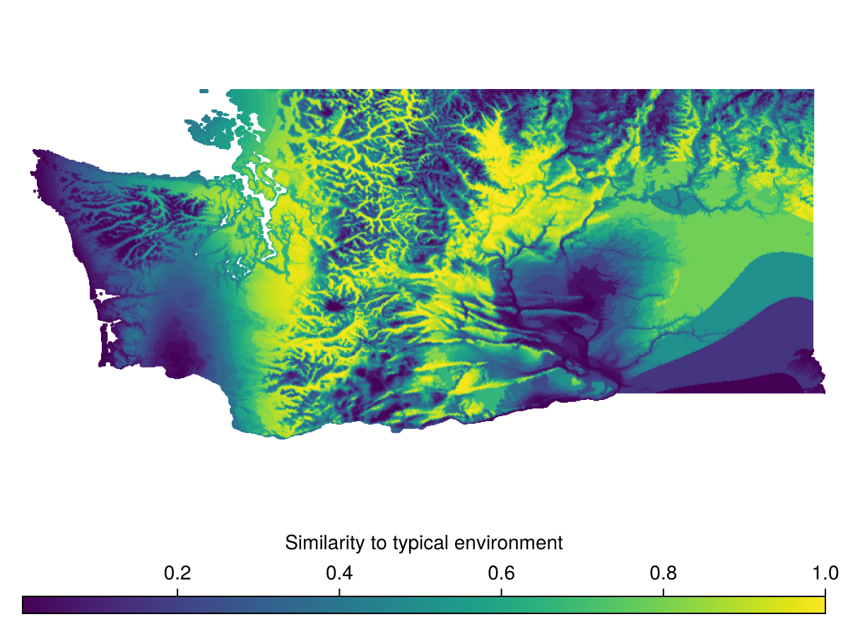
Code for the figure
f = Figure()
ax = Axis(f[1,1], aspect=DataAspect())
hm = heatmap!(ax, mess)
hidedecorations!(ax)
hidespines!(ax)
Colorbar(f[2,1], hm, vertical = false, label="Similarity to typical environment")
Distance to Analog Node
Another metric for climate rarity is comparing the environmental conditions across a domain to the conditions at an existing BiodiversityObservationNetwork.
DistanceToAnalogNode measures the distance of every pixel in the domain to the closest BON site in environmental space.
We can demonstrate this by first sampling a BON
bon = sample(SimpleRandom(), bioclim)BiodiversityObservationNetwork(50 sites via SimpleRandom)and running
dist_to_analog = evaluate(
    DistanceToAnalogNode(),
    bioclim,
    bon
)
🗺️ A 416 × 952 layer with 303225 Float64 cells
Spatial Reference System: +proj=longlat +datum=WGS84 +no_defswhich we can then visualize
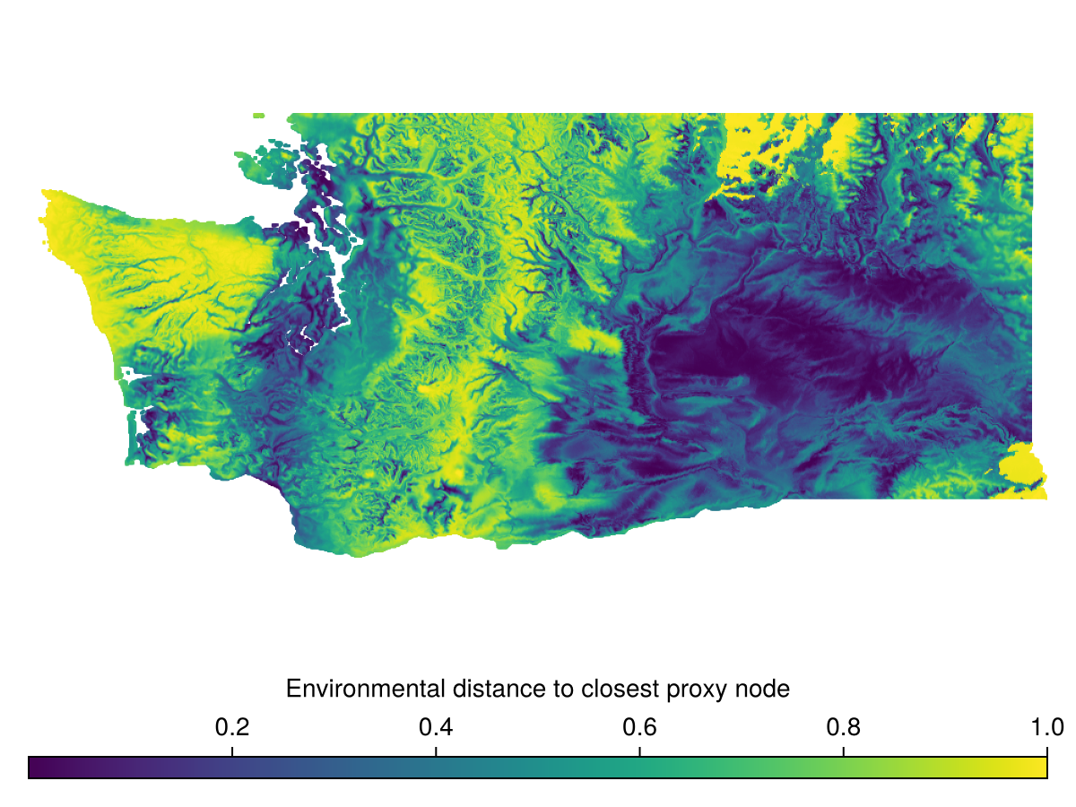
Code for the figure
f = Figure()
ax = Axis(f[1,1], aspect=DataAspect())
hidedecorations!(ax)
hidespines!(ax)
hm = heatmap!(ax, dist_to_analog)
Colorbar(f[2,1], hm, vertical = false, label="Environmental distance to closest proxy node")
Within Range
A simpler method for assessing a BON's coverage in environmental space is WithinRange, which determines if each pixel in the domain is within the extrema of the environmental variables at each BON – i.e. if the environmental conditions at a pixel are at least "bounded" by those at the BON sites.
withinrange = evaluate(
    WithinRange(),
    bioclim,
    bon
)
🗺️ A 416 × 952 layer with 303225 Float64 cells
Spatial Reference System: +proj=longlat +datum=WGS84 +no_defs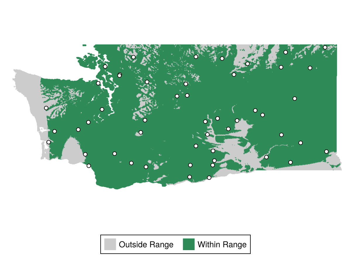
Code for the figure
f = Figure()
ax = Axis(f[1,1], aspect=DataAspect())
hidespines!(ax)
hidedecorations!(ax)
hm = heatmap!(ax, withinrange, colormap=[:grey80, :seagreen4])
scatter!(ax, bon, color=:white, strokewidth=1, strokecolor=:black)
Legend(f[2,1], [PolyElement(color=:grey80), PolyElement(color=:seagreen4)], ["Outside Range", "Within Range"], orientation=:horizontal)
Targeting Rare Climates for Sampling
We can use these climate rarity metrics to target regions of high rarity for sampling.
We will do this using BalancedAcceptance with custom inclusion probabilities, which can be used more generally to target any variable of interest.
We'll start by using DistanceToMedian to compute rarity.
rar = evaluate(
    DistanceToMedian(),
    bioclim
)
🗺️ A 416 × 952 layer with 303225 Float64 cells
Spatial Reference System: +proj=longlat +datum=WGS84 +no_defsWe can sample a BON with inclusion proportional to rarity as follows
bon = sample(BalancedAcceptance(), rar, inclusion = rar)BiodiversityObservationNetwork(50 sites via BalancedAcceptance)Let's visualize this
Code for the figure
f = Figure()
ax = Axis(f[1,1], aspect=DataAspect())
hidespines!(ax)
hidedecorations!(ax)
heatmap!(ax, rar)
scatter!(ax, bon, color=:white, strokewidth=1, strokecolor=:black)
Colorbar(f[2,1], hm, vertical = false, label="Distance to Median Environment")
We see the points are generally more concentrated toward the left side of the map, where the environmental conditions are more rare.
Pragmatically, this may not be skewed "enough" toward rare regions, so we can adjust the relative inclusion probabilities by applying an exponential transformation with a parameter
αs = [1,3,5,10]
bons = [sample(BalancedAcceptance(), rar, inclusion=exp.(αs[i] * rar)) for i in eachindex(αs)]
4-element Vector{BiodiversityObservationNetwork{CartesianIndex{2}}}:
BiodiversityObservationNetwork(50 sites via BalancedAcceptance)
BiodiversityObservationNetwork(50 sites via BalancedAcceptance)
BiodiversityObservationNetwork(50 sites via BalancedAcceptance)
BiodiversityObservationNetwork(50 sites via BalancedAcceptance)We can then visualize to see the impact of this transform
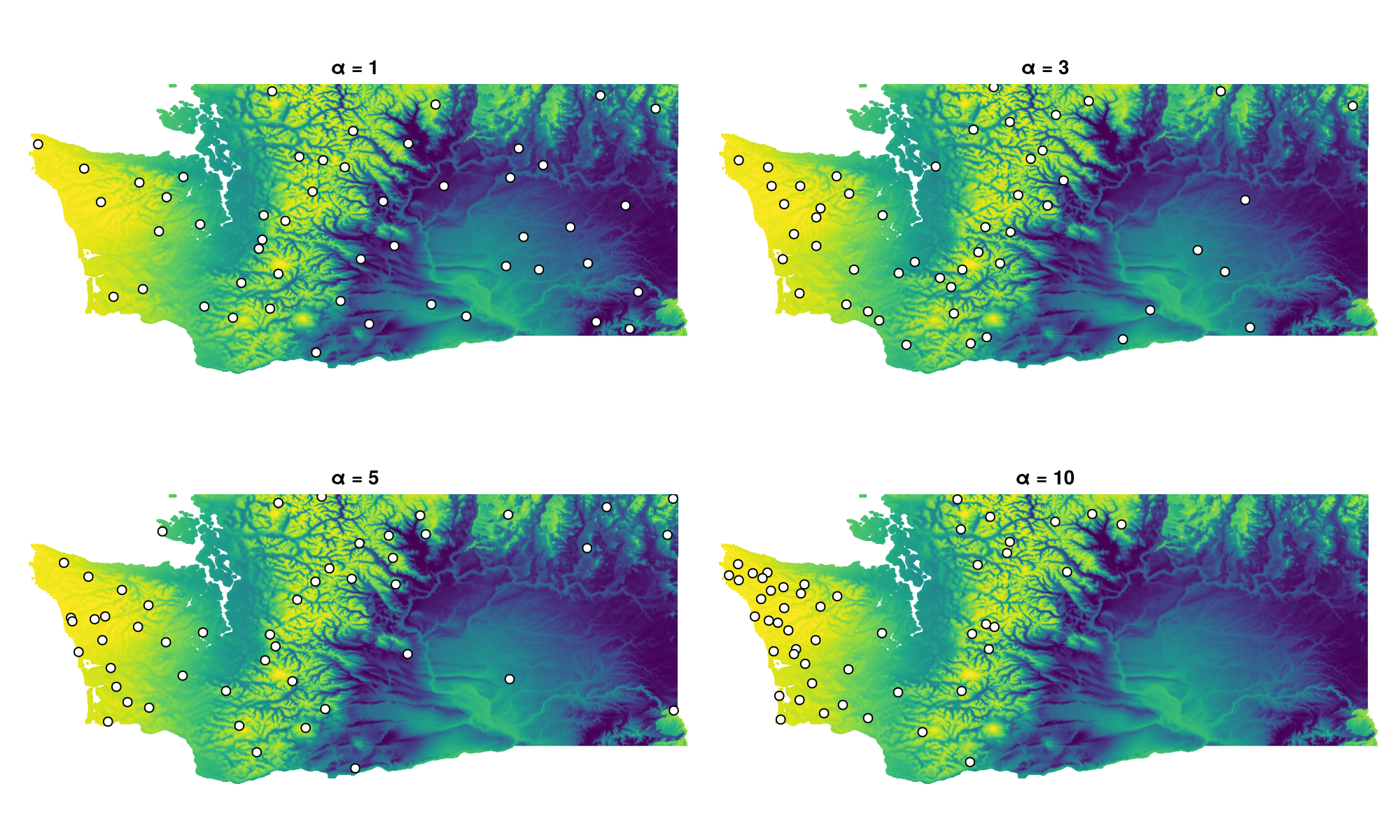
Code for the figure
f = Figure(size=(1000, 600))
axes = [Axis(f[ci[2],ci[1]], title = "α = $(αs[i])", aspect=DataAspect()) for (i,ci) in enumerate(CartesianIndices((1:2,1:2)))]
for i in eachindex(axes)
    heatmap!(axes[i], rar)
    scatter!(axes[i], bons[i], color=:white, strokewidth=1, strokecolor=:black)
end
hidespines!.(axes)
hidedecorations!.(axes)
Next steps
In the next tutorial, we'll cover how to evaluate the spatial balance and environmental representativeness of a particular BON.