Evaluating BON Design

BiodiversityObservationNetworks.jl contains several utilities for measuring properties of a BON. These properties can be split into two categories: (1) properties that measure spatial balance and (2) properties that measure environmental balance.

Let's load the packages and a couple functions from StatsBase

using BiodiversityObservationNetworks
using BiodiversityObservationNetworks.StatsBase: mean, std
using CairoMakie
using SpeciesDistributionToolkit

Random.TaskLocalRNG()

There are three metrics for evaluating BON design: two measure the spatial balance of a sample (MoransI and VoronoiVariance), and one measures how representative the environmental conditions at BON are relative to the domain being sampled (``).

Moran's I

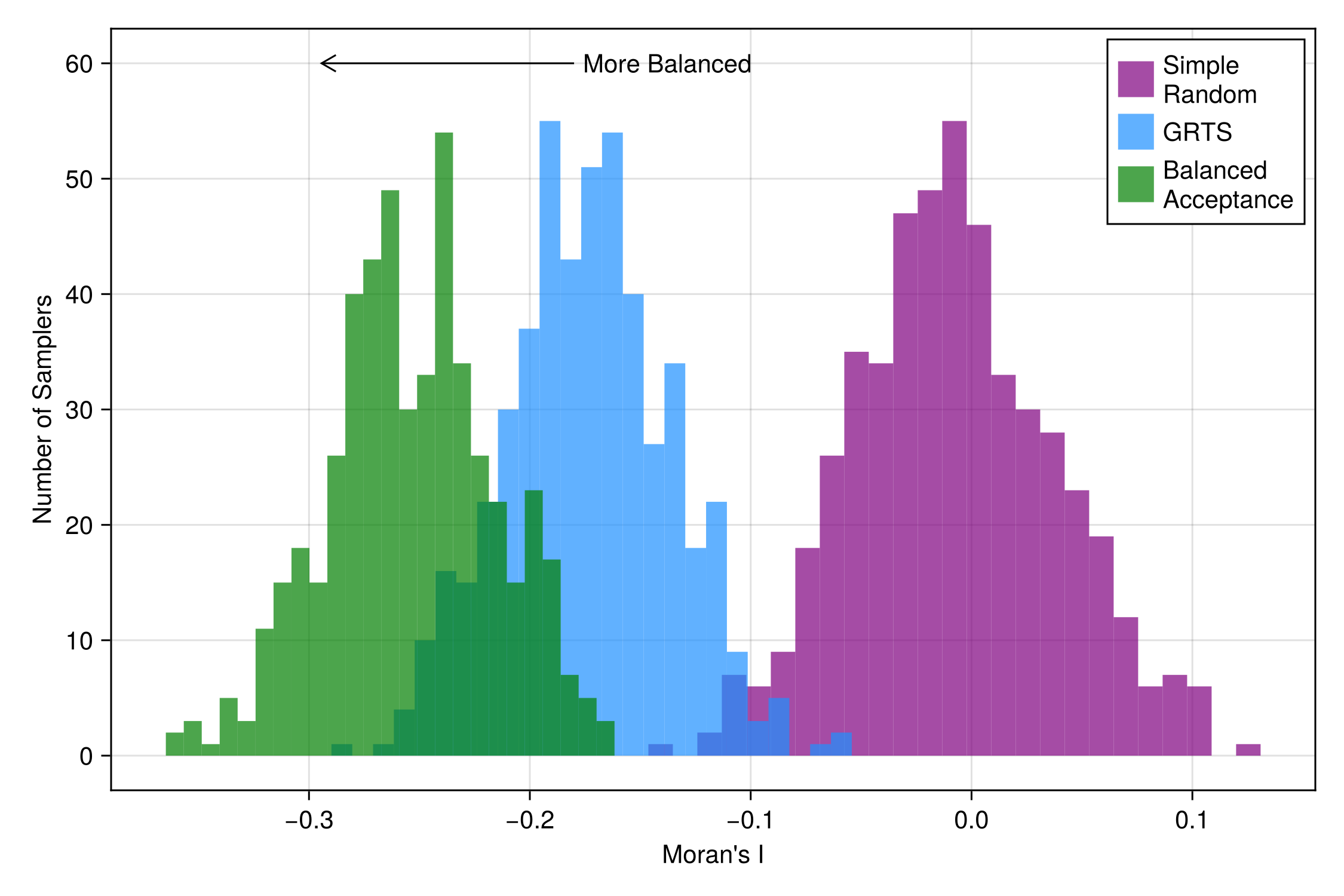
MoransI is a metric that calculates spatial autocorrelation of the sample indicator variable across the domain (1 if a site is sampled, 0 otherwise). Negative values indicate spatial inhibition (spread), which is desired for balanced sampling. This version was specifcally proposed by (Tillé et al., 2025).

For these examples, we'll use a 30 x 30 matrix of zeros as our domain, but any domain will work here

domain = zeros(30, 30);

Let's compare spatial balance (using MoransI) for three different sampling algorithms: (1) SimpleRandom, (2) BalancedAcceptance and (3) GRTS.

We'll use 500 random BON samples per sampling method

reps = 500

500

And use in-line loops to record Moran's $\mathcal{I}$ across 500 random BONs across our domain

grts_I = [spatialbalance(MoransI(), domain, sample(GRTS(), domain)) for r in 1:reps];
bas_I = [spatialbalance(MoransI(), domain, sample(BalancedAcceptance(), domain)) for r in 1:reps];
srs_I =  [spatialbalance(MoransI(), domain, sample(SimpleRandom(), domain)) for r in 1:reps];

And visualize the scores of each sampler.

Code for the figure

f = Figure(size=(750,500))
NUM_BINS = 25
ax = Axis(f[1,1], xlabel = "Moran's I", ylabel = "Number of Samplers")
hist!(ax, srs_I, color=(:purple, 0.7), bins=NUM_BINS, label = "Simple\nRandom")
hist!(ax, grts_I, color=(:dodgerblue, 0.7), bins=NUM_BINS, label = "GRTS")
hist!(ax, bas_I, color=(:green, 0.7), bins=NUM_BINS, label = "Balanced\nAcceptance")
annotation!(ax, 200, 0, -0.3, 60,
    text = "More Balanced",
    style = Ann.Styles.LineArrow()
)
axislegend(position = :rt)

As we can see (and is consistent with the results in the literature that developed these samplering algorithms), GRTS is more spatially balanced than Simple Random Sampling, but is outperformed by Balanced Acceptance Sampling.

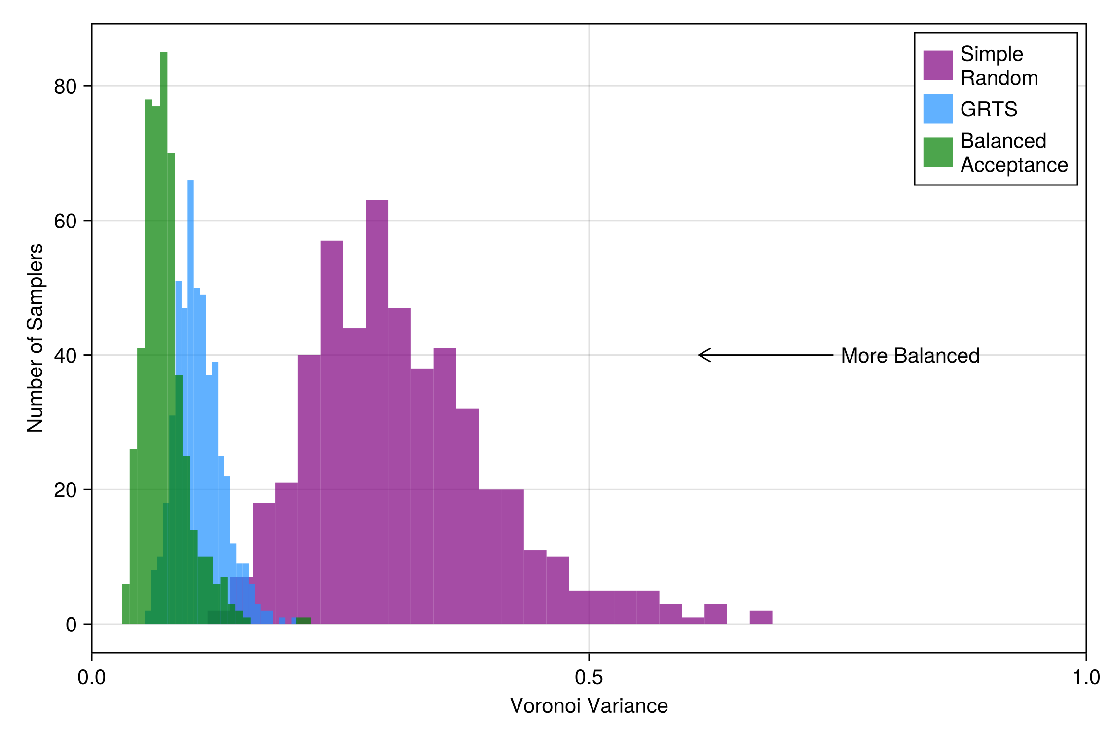
VoronoiVariance

An alternative method for evaluating spatial balance is by using the Voronoi tesselation, which splits the domain into a series of polygons, where the $i$-th polygon consists of all points in the plane whose nearest node in bon is the $i$-th node.

These polygons can then be used to assess the spatial balance of a sample. In an ideally balanced sample, the sum of the inclusion probabilities within each polygon $i$ would equal 1, because in expectation exactly one unit would be sampled in that region.

If we define $v_i$ as the total inclusion probability across Voronoi polygon i, i.e.

$$v_i={\int }_{j\in i}{\pi }_{j}dj$$

then we can assess the spatial balance of a sample by measuring the distance of $v_i$ from 1 for each polygon.

(Grafström, 2025) proposes the metric B, defined as

$$B=\frac{1}{n}\sum _{i=1}^n(v_i-1{)}^2$$

to measure spatial balance, where smaller values indicate better spatial balance.

We'll now compare VoronoiVariance across samplers in the same way as above:

grts_vv = [spatialbalance(VoronoiVariance(), domain, sample(GRTS(), domain)) for r in 1:reps];
bas_vv = [spatialbalance(VoronoiVariance(), domain, sample(BalancedAcceptance(), domain)) for r in 1:reps];
srs_vv =  [spatialbalance(VoronoiVariance(), domain, sample(SimpleRandom(), domain)) for r in 1:reps];

and visualize

Code for the figure

f = Figure(size=(750,500))
NUM_BINS = 25
ax = Axis(f[1,1], xlabel = "Voronoi Variance", ylabel = "Number of Samplers")
hist!(ax, srs_vv, color=(:purple, 0.7), bins=NUM_BINS, label = "Simple\nRandom")
hist!(ax, grts_vv, color=(:dodgerblue, 0.7), bins=NUM_BINS, label = "GRTS")
hist!(ax, bas_vv, color=(:green, 0.7), bins=NUM_BINS, label = "Balanced\nAcceptance")
annotation!(ax, 150, 0, 0.6, 40,
    text = "More Balanced",
    style = Ann.Styles.LineArrow()
)
xlims!(ax, 0,1)
axislegend(position = :rt)

and again we see that GRTS is more spatially balanced than Simple Random Sampling, but is outperformed by Balanced Acceptance Sampling.

JensenShannon

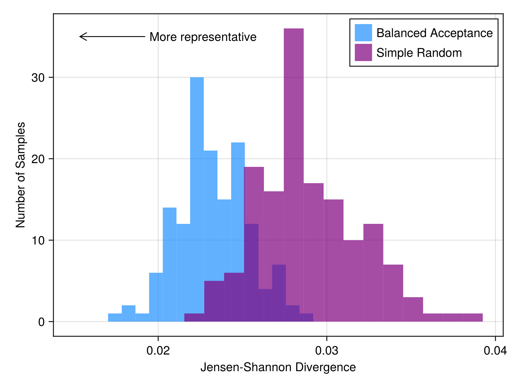
The final evaluation metric is for computing how representative a BiodiversityObservationNetwork is of the environmental variables across the domain using Jensen-Shannon divergence, a method for measuring the distance between two distributions.

Here we will use bioclimatic variables in Washington State as an example

aoi = getpolygon(PolygonData(OpenStreetMap, Places), place = "Washington State")

FeatureCollection with 1 features, each with 10 properties

We can then load the 19 Bioclimatic variables from CHELSA as follows.

bioclim = [SDMLayer(RasterData(CHELSA1, BioClim); SpeciesDistributionToolkit.SimpleSDMPolygons.boundingbox(aoi)..., layer = i) for i in 1:19]

19-element Vector{SimpleSDMLayers.SDMLayer{Int16}}:
 🗺️  A 416 × 952 layer (355723 Int16 cells)
 🗺️  A 416 × 952 layer (355723 Int16 cells)
 🗺️  A 416 × 952 layer (355723 Int16 cells)
 🗺️  A 416 × 952 layer (355723 Int16 cells)
 🗺️  A 416 × 952 layer (355723 Int16 cells)
 🗺️  A 416 × 952 layer (355723 Int16 cells)
 🗺️  A 416 × 952 layer (355723 Int16 cells)
 🗺️  A 416 × 952 layer (355723 Int16 cells)
 🗺️  A 416 × 952 layer (355723 Int16 cells)
 🗺️  A 416 × 952 layer (355723 Int16 cells)
 🗺️  A 416 × 952 layer (355723 Int16 cells)
 🗺️  A 416 × 952 layer (355723 Int16 cells)
 🗺️  A 416 × 952 layer (355723 Int16 cells)
 🗺️  A 416 × 952 layer (355723 Int16 cells)
 🗺️  A 416 × 952 layer (355723 Int16 cells)
 🗺️  A 416 × 952 layer (355723 Int16 cells)
 🗺️  A 416 × 952 layer (355723 Int16 cells)
 🗺️  A 416 × 952 layer (355723 Int16 cells)
 🗺️  A 416 × 952 layer (355723 Int16 cells)

And mask them to just Washington state.

mask!(bioclim, aoi)

19-element Vector{SimpleSDMLayers.SDMLayer{Int16}}:
 🗺️  A 416 × 952 layer (303225 Int16 cells)
 🗺️  A 416 × 952 layer (303225 Int16 cells)
 🗺️  A 416 × 952 layer (303225 Int16 cells)
 🗺️  A 416 × 952 layer (303225 Int16 cells)
 🗺️  A 416 × 952 layer (303225 Int16 cells)
 🗺️  A 416 × 952 layer (303225 Int16 cells)
 🗺️  A 416 × 952 layer (303225 Int16 cells)
 🗺️  A 416 × 952 layer (303225 Int16 cells)
 🗺️  A 416 × 952 layer (303225 Int16 cells)
 🗺️  A 416 × 952 layer (303225 Int16 cells)
 🗺️  A 416 × 952 layer (303225 Int16 cells)
 🗺️  A 416 × 952 layer (303225 Int16 cells)
 🗺️  A 416 × 952 layer (303225 Int16 cells)
 🗺️  A 416 × 952 layer (303225 Int16 cells)
 🗺️  A 416 × 952 layer (303225 Int16 cells)
 🗺️  A 416 × 952 layer (303225 Int16 cells)
 🗺️  A 416 × 952 layer (303225 Int16 cells)
 🗺️  A 416 × 952 layer (303225 Int16 cells)
 🗺️  A 416 × 952 layer (303225 Int16 cells)

The API for [JensenShannon] is similar to other evaluation utilties:

bon = sample(SimpleRandom(), bioclim)
js = evaluate(JensenShannon(), bioclim, bon)

0.05318806815211255

We can then compare BalancedAcceptance to SimpleRandom:

nreps = 150
bas = [evaluate(JensenShannon(), bioclim, sample(BalancedAcceptance(100), bioclim)) for i in 1:nreps];
srs = [evaluate(JensenShannon(), bioclim, sample(SimpleRandom(100), bioclim)) for i in 1:nreps];

and visualize

Code for the figure

f = Figure()
ax = Axis(f[1,1], xlabel = "Jensen-Shannon Divergence", ylabel = "Number of Samples")
hist!(bas, color=(:dodgerblue, 0.7), label = "Balanced Acceptance")
hist!(srs, color=(:purple, 0.7), label="Simple Random")
annotation!(ax, 150, 0, 0.015, 35,
    text = "More representative",
    style = Ann.Styles.LineArrow()
)
axislegend(position = :rt)

Note that the spatially balanced sampler, BalancedAcceptance, is more environmentally representative than SimpleRandom.