Getting Started with BiodiversityObservationNetworks.jl

BiodiversityObservationNetworks.jl (BONs.jl) is a Julia package for selecting sites for spatial sampling, typically in the context of ecological or biodiversity sampling design. The purpose of this package is to provide a high-level, extensible, modular interface to the selection of sampling point for biodiversity processes in space. BONs.jl implements a variety of algorithms for site selection, including stratified and spatially balanced sampling, and enables adaptive sampling based on model-based estimates of uncertainty or the locations of legacy sampling sites. It also includes a variety of utilities for quantifying a sample's spatial balance and how representative a sample is of auxiliary environmental variables.

In this tutorial, we will cover the basics of how to use BiodiversityObservationNetworks.jl. Let's start by loading the package.

using BiodiversityObservationNetworks
using CairoMakie

Installing and loading

To install BONS.jl, use either Pkg

using Pkg; Pkg.add("BiodiversityObservationNetworks")

or the REPL Pkg mode.

Then load it via

using BiodiversityObservationNetworks

Your first sample

The core function in BONs.jl is sample. sample works by taking a sampling algorithm (a type of BONSampler) and a sampling domain, which represents the region from which to select sampling points.

The core pattern for selecting sites is to call sample(algorithm, domain), with additional arguments available depending on the specific algorithm used.

BONs.jl supports a variety of domains, including raster and vector data. The simplest domain is a plain Julia Matrix:

mat = rand(50, 50);

The simplest sampler is SimpleRandom, which randomly selects sites without replacement.

result = sample(SimpleRandom(), mat)

BiodiversityObservationNetwork(50 sites via SimpleRandom)

sample returns a BiodiversityObservationNetwork, which stores the indices of the selected sites within the domain, their (geospatial, if applicable) coordinates, and the values of auxiliary variables at the selected sites (if available).

By default, all algorihtms will select 50 sites. This is changed simply by passing an integer value to the sampler. For example

result = sample(SimpleRandom(10), mat)

BiodiversityObservationNetwork(10 sites via SimpleRandom)

will yield 10 selected sites.

Visualizing Results

To plot the results, we use Makie, a feature-rich package in Julia for data visualization.

BONs.jl functionality for Makie relies on a Julia extension, meaning it is only activated if Makie is loaded in the same environment.

Makie can be installed and loaded similar to above. Makie provides various "backends", for different types of plotting. Here we will used CairoMakie, which is the backend for publication-quality graphics. You can learn more about Makie and the different available backends here

using CairoMakie

A BON can then be visualized with the scatter method.

scatter(result)

All typical keyword arguments can be passed to scatter to customize the result, e.g.

scatter(result; color = :green, marker = :star5, markersize = 15, axis=(;aspect=1))

Understanding the BiodiversityObservationNetwork type

The BiodiversityObservationNetwork type stores a variety of information about the sample.

The first is sites, which are the indices in the original domain for the selected sites (typically a vector of CartesianIndexs)

result.sites

10-element Vector{CartesianIndex{2}}:
 CartesianIndex(40, 14)
 CartesianIndex(26, 40)
 CartesianIndex(19, 28)
 CartesianIndex(49, 28)
 CartesianIndex(22, 2)
 CartesianIndex(12, 49)
 CartesianIndex(10, 42)
 CartesianIndex(47, 32)
 CartesianIndex(23, 43)
 CartesianIndex(35, 22)

BiodiversityObservationNetwork also have a field called coordinates

result.coordinates

2×10 Matrix{Int64}:
 40  26  19  49  22  12  10  47  23  35
 14  40  28  28   2  49  42  32  43  22

At first, this may seem to be redundant as the same information is stored in sites, but this allows for storing both the Cartesian indices of selected sites a raster, and their corresponding geospatial coordinates when using supported geospatial domains from SpeciesDistributionToolkit.jl. You can read more about the different types of domains in the next tutorial.

When the domain is a single matrix (like mat), the auxiliary variables in the BiodiversityObservationNetwork are simply the values of the original matrix at each selected, which are stored in a matrix called features

result.features

1×10 Matrix{Float64}:
 0.480072  0.360887  0.840594  0.955736  0.406768  0.255568  0.00896954  0.484482  0.47109  0.535093

We can see that the first feature is the value of the domain at the first site

mat[result.sites[begin]]

0.48007212600054794

When using multiple rasters/matrices as a domain, the auxiliary variables are the values across each of those rasters. For example,

multilayer_domain = [rand(30,20) for i in 1:5]
multilayer_result = sample(SimpleRandom(10), multilayer_domain)

BiodiversityObservationNetwork(10 sites via SimpleRandom)

Will yield a matrix of auxiliary variables of dimension 5 x 10 (for 5 auxiliary variables at each of 10 sites)

multilayer_result.features

5×10 Matrix{Float64}:
 0.848805   0.379682  0.708246  0.451363   0.075318  0.519829  0.676904   0.49055   0.340822  0.361665
 0.868744   0.720612  0.601528  0.385875   0.406657  0.325258  0.535672   0.270134  0.846874  0.0627669
 0.830064   0.339126  0.404188  0.0217998  0.464919  0.5811    0.966597   0.828651  0.11021   0.0928874
 0.0517573  0.378896  0.350533  0.347309   0.702662  0.427639  0.0949562  0.655809  0.279756  0.600263
 0.833471   0.142943  0.107299  0.42759    0.796693  0.321331  0.28882    0.642778  0.794978  0.793987

Masking sites

Use the mask keyword to restrict sampling to a subset of the grid. A true value in the mask means the cell is valid (i.e. can be included in a sampled result).

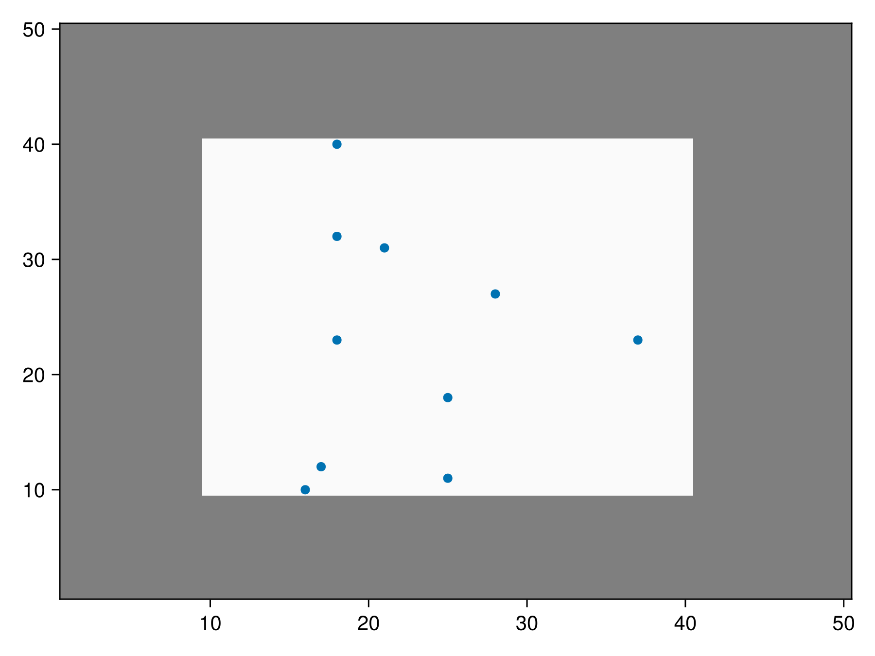
As an example, lets build a mask that restricts points to the center 30x30 region of a 50x50 matrix.

mask = falses(50, 50)
mask[10:40, 10:40] .= true   # only sample the central region
result_masked = sample(SimpleRandom(10), mat; mask = mask)

BiodiversityObservationNetwork(10 sites via SimpleRandom)

We can plot the valid region in white and the invalid region in grey to verify that all the coordinates fall in the valid region of the mask.

Code for the figure

f = Figure()
ax = Axis(f[1,1])
heatmap!(ax, mask, colormap=[:grey50, :grey98])
scatter!(ax, result_masked)

Custom Inclusion Probabilities

Up until this point, we have been using the SimpleRandom sampler, which draws sampling locations with equal probability, without replacement. For a variety of reasons, we may want the initial probability that a site is included to vary, so some locations are more likely to be included than others. Many sampling algorithms, including SimpleRandom, support this functionality.

For example, lets make it so the inclusion probability increases as we move from left to right across the domain. This can be done via

inclusion_probability = [1.15^i for i in 1:50, j in 1:50];

Let's plot this matrix to verify this is what we get

heatmap(inclusion_probability)

Now we can sample with sites with these custom inclusion probabilities using the inclusion keyword argument

result = sample(SimpleRandom(), inclusion_probability, inclusion = inclusion_probability)

BiodiversityObservationNetwork(50 sites via SimpleRandom)

and very can verify the selected points are skewed more toward the right side of the domain

scatter(result)

Inclusion probabilities as weights

Formally, inclusion probabilities are defined as the unit $i$ having inclusion probability ${\pi }_i$, and the expected number of total units included in the sample is $\sum _i{\pi }_i$.

In BONs.jl, the desired sample size $N$ are defined as properties of the BONSampler. As a result, we take any arbitrary set of positive values provided as inclusion probabilities, and renormalize them such that $\sum _i{\pi }_i=N$, rather than enforcing that they sum to $N$ to begin with.

Note that the inclusion probability matrix doesn't have to be the domain. Different inclusion probabilities and domains can be used as long as they are compatible, meaning they are equally sized matrices, or a SDMLayer with matching size, extent, and coordinate-representation-system (crs).

For example

result = sample(SimpleRandom(), rand(50, 50); inclusion = inclusion_probability)

BiodiversityObservationNetwork(50 sites via SimpleRandom)

is also valid because the domain is also a 50 x 50 matrix.

Custom Inclusion Probabilities with Masks

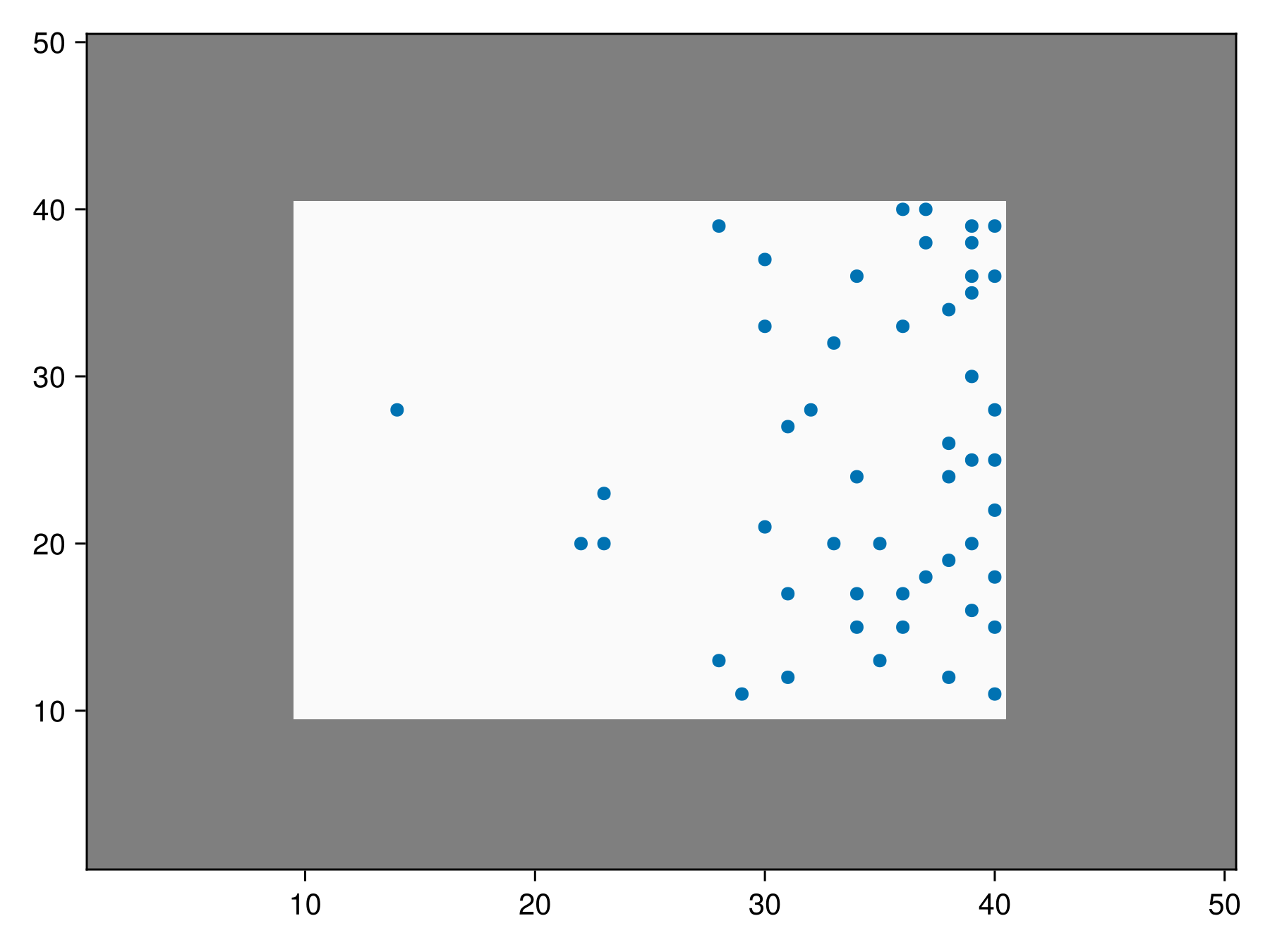
Note that both masks and inclusion probabilities can be used together.

inclusion_masked_bon = sample(SimpleRandom(), rand(50, 50), inclusion = inclusion_probability, mask = mask)

BiodiversityObservationNetwork(50 sites via SimpleRandom)

We can visualize this to show the middle masked region is the only valid region, but points are still more likely on the right side.

Code for the figure

fig = Figure()
ax = Axis(fig[1,1])
heatmap!(ax, mask, colormap=[:grey50, :grey98])
scatter!(ax, inclusion_masked_bon)

In this case, any inclusion probability in masked regions is ignored and inclusion weights are renormalized only using unmasked regions (see note above).

Next Steps

This covers the basic functionality of BONs.jl. More advanced functionality is explored in the following tutorials, which we recommend following in the below order:

• Geospatial Domains with SpeciesDistributionToolkit

• Targeting samplers toward rare climates

• Evaluating selected sites

In addition, full descriptions of each of the supported algorithms for sampling can be found here.

Description of the various utilities in BONs.jl can be found here, and a design document describing how the internals of the package are designed (primarily aimed for contributors to the package) can be found here.