Geospatial Domains in BONs.jl

In most contexts, selecting spatial sampling sites requires choosing a set of locations from an explicitly geospatial domain, associated with geographical coordinates. BONs.jl supports both raster and vector geospatial domains through integration with SpeciesDistributionToolkit.jl (SDT.jl).

Here, we will explore how this integration works through examples.

SDT.jl integration is included as a Julia extension, meaning each package must be installed and loaded in order to enable functionality.

using BiodiversityObservationNetworks
using SpeciesDistributionToolkit

A Geospatial Raster Domain

A natural extension of the Matrix domain, the simplest domain supported by BONs.jl, is using a geospatial raster. A raster is also just a matrix of values, but also containing additional metadata that associates each element of the matrix with a geographic location.

BONs.jl supports this through the SDMLayer type from SpeciesDistributionToolkit.jl.

Let's load an example SDMLayer to understand the basics of how the SDMLayer type works. Full documentation of what data sources are available in SDT, and how they can be manipulated, is available in the SDT.jl documentation. The below lines load a raster that contains the average annual temperature for Corsica.

spatial_extent = (left = 8.412, bottom = 41.325, right = 9.662, top = 43.060) # the longitude/latitude extent of Corsica
temp = SDMLayer(RasterData(CHELSA1, AverageTemperature); spatial_extent...,)

🗺️  A 209 × 151 layer with 14432 Int16 cells
   Spatial Reference System: +proj=longlat +datum=WGS84 +no_defs

We can plot it using heatmap from Makie to visualize

Code for the figure

f = Figure()
ax = Axis(f[1,1], aspect=DataAspect())
hm = heatmap!(ax, temp, colormap=:OrRd)

Sampling from this SDMLayer works exactly like sampling from a matrix. For example, we can use the SimpleRandom as follows:

bon = sample(SimpleRandom(), temp)

BiodiversityObservationNetwork(50 sites via SimpleRandom)

Which we can then plot

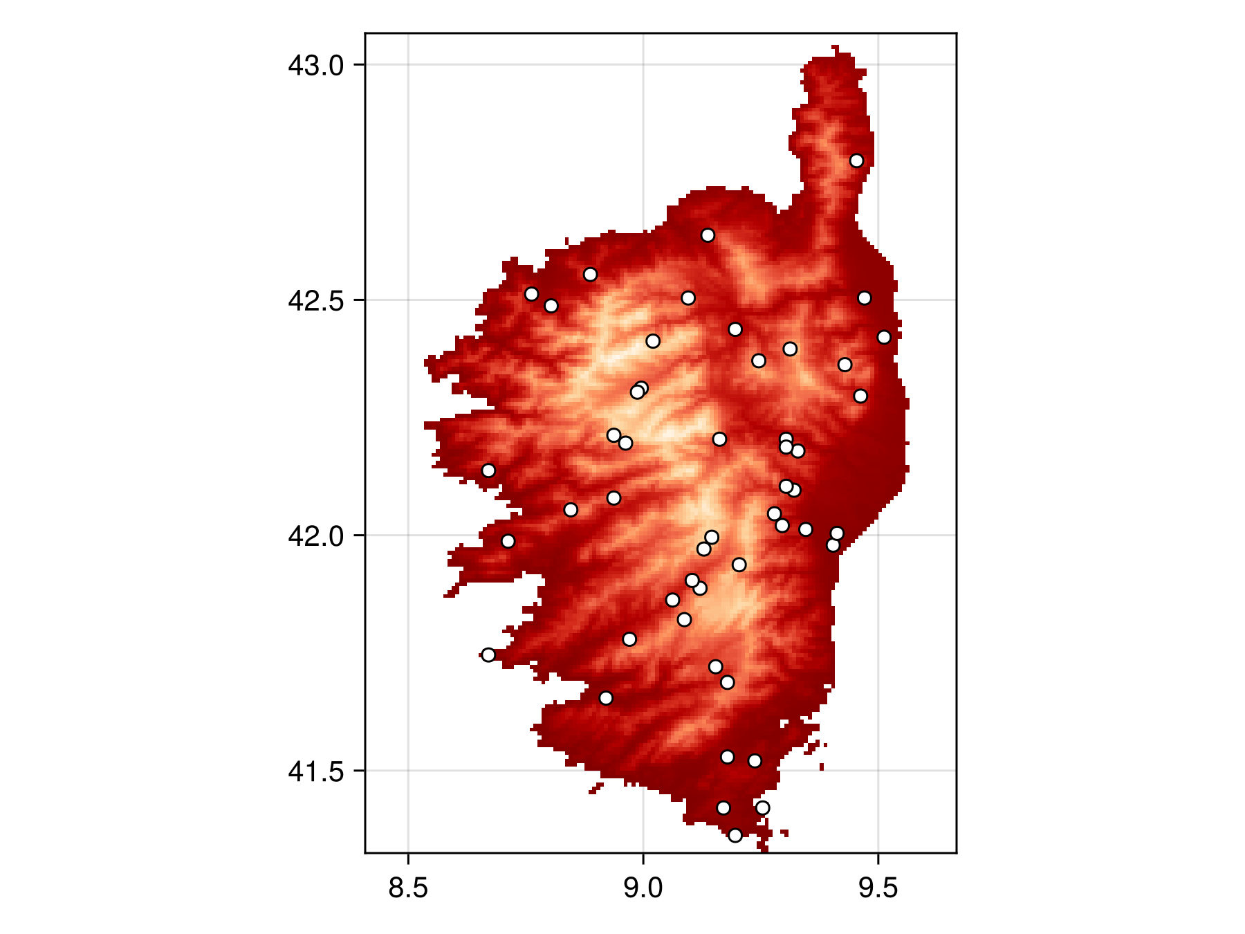
Code for the figure

f = Figure()
ax = Axis(f[1,1], aspect=DataAspect())
hm = heatmap!(ax, temp, colormap=:OrRd)
scatter!(ax, bon, color=:white, strokewidth=1, strokecolor=:black)

Note that there are regions in the raster (the water of surrouding Corsica) that have no value. Samplers will automatically avoid sampling sites in those regions –- only pixels with valid data are considered for sampling.

Masking Geospatial Rasters

As we've just seen, regions without valid pixel data are automatically ignored. However, we can mask addition pixels using the mask keyword.

For a SDMLayer domain, the type of object we pass to mask can either be (1) a matrix with the same size as the SDMLayer domain. or (2) another SDMLayer with the same size, extent, and resolution as the SDMLayer used as the domain,

Here we will provide an example of both forms to mask out the center region of Corsica.

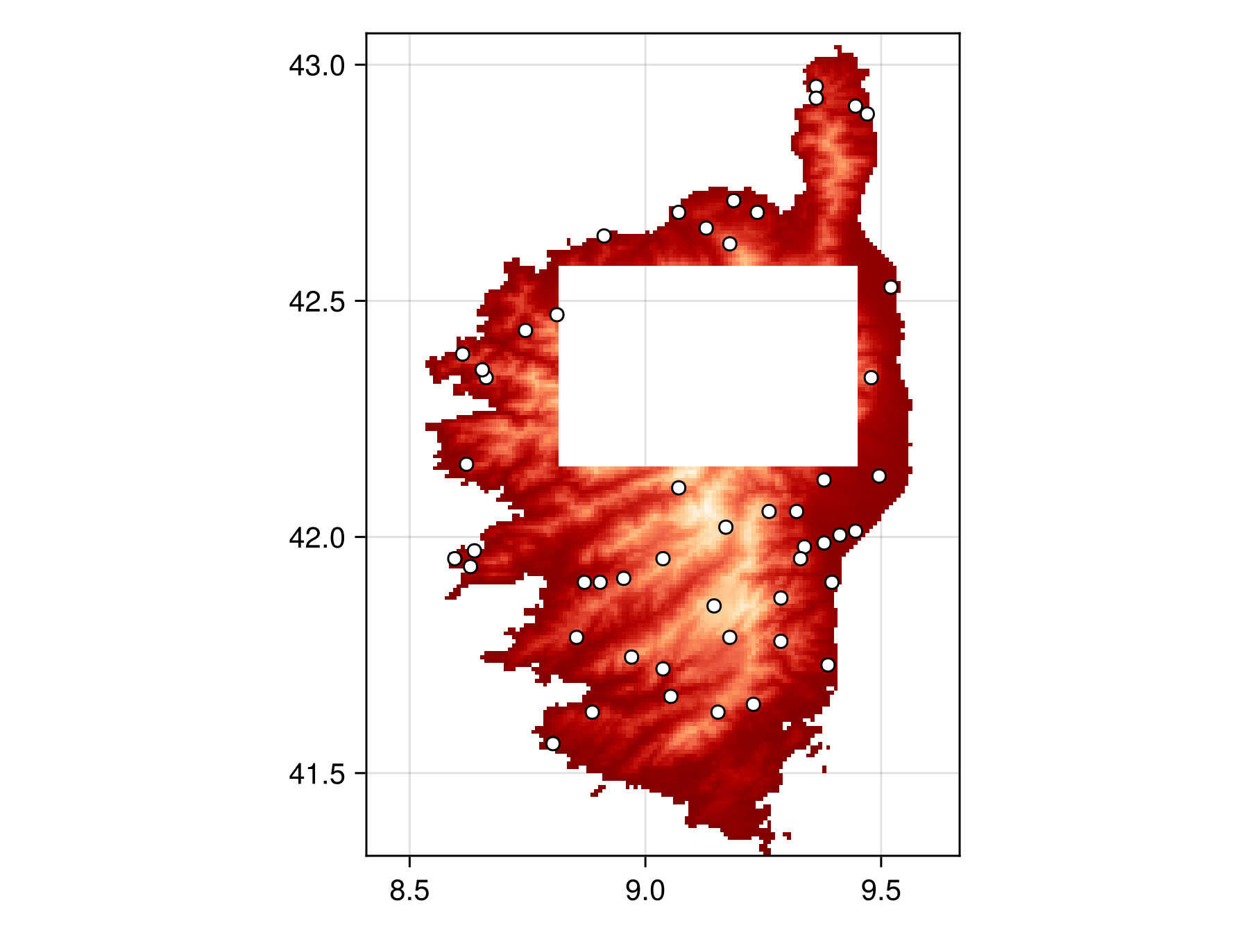
Masking a SDMLayer with a matrix

Let's construct our mask by first creating a matrix of all ones that is the same size as our SDMLayer.

matrix_mask = ones(size(temp));

And now set a box in the middle to 0s to make it "off-limits" for the sampler

matrix_mask[100:150, 50:125] .= false;

Now we can sample

masked_bon = sample(SimpleRandom(), temp, mask = matrix_mask)

BiodiversityObservationNetwork(50 sites via SimpleRandom)

And plot to verify points are all outside the masked region.

Code for the figure

f = Figure()
ax = Axis(f[1,1], aspect=DataAspect())
hm = heatmap!(ax, temp2, colormap=:OrRd)
scatter!(ax, masked_bon, color=:white, strokewidth=1, strokecolor=:black)

Hiding masked regions in the SDMLayer

Note that we have done a bit of trickery on the SDMLayer to hide the masked pixels in the plot. This was done by running

temp2 = copy(temp)
temp2.indices[findall(iszero, matrix_mask)] .= 0

and plotting temp2, which we sneakily hid from the code above to avoid confusion and unnecessary detail.

Note this has no effect on the actual sampling of the sites, it is simply for visualization purposes to verify no sampled sites fall within the mask.

Masking a SDMLayer with another SDMLayer

SDMLayers can also be used as masks, assuming they have the same size, extent, and crs as the domain.

SDMLayer masks only mask out the regions that are set as invalid pixels, regardless of the pixel value. Unlike a matrix mask, the whether the value of an SDMLayer's pixel is not what is used to determine if a site is masked. SDMLayers have a separate field called indices, which determine what pixels are valid. The indices field is what is used to mask sampling sites

To construct an SDMLayer mask, we start by constructing a copy of our temp

layer_mask = copy(temp)

🗺️  A 209 × 151 layer with 14432 Int16 cells
   Spatial Reference System: +proj=longlat +datum=WGS84 +no_defs

The validity of each pixel is stored in the indices field of an SDM. To construct a mask, we can run the lines

layer_mask.indices[100:150, 50:125] .= 0; # set center of Corsica to 0

which will remove the center region of Corsica from consideration.

We can visualize the new layer mask

Code for the figure

f = Figure()
ax = Axis(f[1,1], aspect=DataAspect())
hm = heatmap!(ax, layer_mask, colormap=:OrRd)

We can then pass the layer_mask to the mask keyword argument as normal:

masked_bon = sample(SimpleRandom(), temp, mask = layer_mask)

BiodiversityObservationNetwork(50 sites via SimpleRandom)

and plot to verify the masking works

Code for the figure

f = Figure()
ax = Axis(f[1,1], aspect=DataAspect())
hm = heatmap!(ax, layer_mask, colormap=:OrRd)
scatter!(ax, masked_bon, color=:white, strokewidth=1, strokecolor=:black)

Custom Inclusion Probabilities with Geospatial Rasters

When using custom inclusion probabilities with an SDMLayer domain, things work very similarly to masking. Either (1) a matrix of the same size or (2) an SDMLayer with the same size, extent and crs can be used as inclusion probabilities.

A inclusion probabilities matrix with an SDMLayer domain.

Let's construct inclusion probabilities where the right side is more likely to be included, as we did in the first tutorial.

inclusion_probabilies = [1.15^j for i in 1:size(temp,1), j in 1:size(temp, 2)];

x/y vs. longitude/latitude

You may notice above that to make inclusion increase as we go right, we use 1.15^j, where as in the first tutorial we used 1.15^i.

This is because in a matrix, i (the first axis) typically corresponds to the horizontal axis, but in a raster, j (the second axis) typically corresponds to the horizontal/longitude axis.

This is a result of decisions that people made before many of us were born and that we will all likely have to live with until we are all dead. That's just how it is.

We can then use this with the inclusion keyword argument

inclusion_bon = sample(SimpleRandom(), temp, inclusion = inclusion_probabilies)

BiodiversityObservationNetwork(50 sites via SimpleRandom)

and visualize to confirm it worked

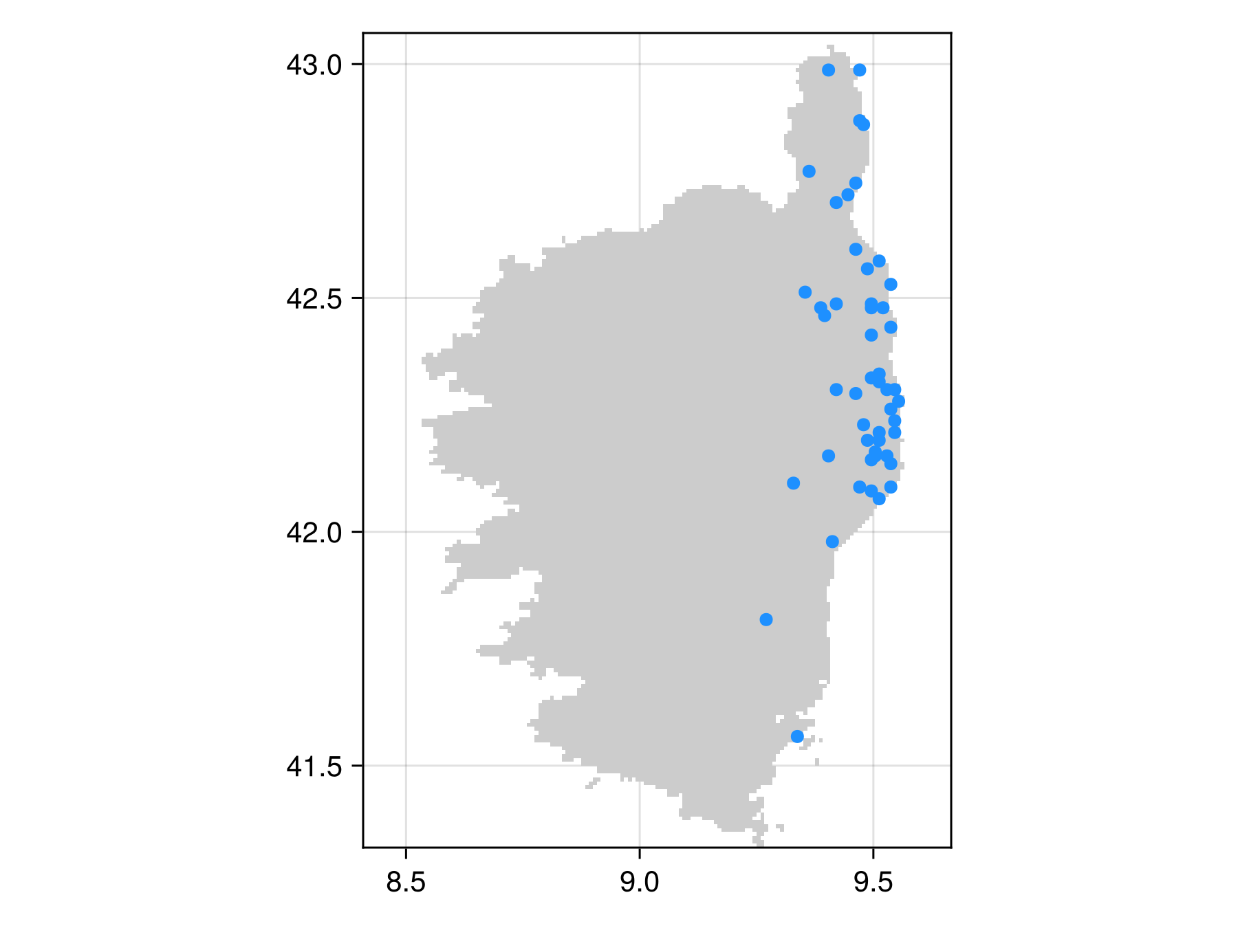
Code for the figure

f = Figure()
ax = Axis(f[1,1], aspect=DataAspect())
heatmap!(ax, temp, colormap=[:grey80])
scatter!(inclusion_bon, color=:dodgerblue)

Using a geospatial vector as a domain

SpeciesDistributionToolkit also supports various types of geospatial vector data (e.g. polygons) as both domains and masks.

Let's start by getting a polygon of the Island of Montréal.

montreal = getpolygon(PolygonData(OpenStreetMap, Places); place = "Island of Montreal")

FeatureCollection with 1 features, each with 10 properties

We can visualize this with either the poly method (to have it filled in), or the lines method (to just show the outline)

poly(montreal)

This can on its own, be used as a domain:

poly_bon = sample(SimpleRandom(), montreal)

BiodiversityObservationNetwork(50 sites via SimpleRandom)

which we can then visualize

Code for the figure

fig = Figure()
ax = Axis(fig[1,1])
poly!(montreal)
scatter!(poly_bon, color=:white, strokewidth=1, strokecolor=:black)

Masking polygons with polygons

We can also use a polygon from SDT as a mask.

Let's download the region that are formally within the Ville de Montreal's jurisdiction region as a polygon

ville_de_m = getpolygon(PolygonData(OpenStreetMap, Places); place = "Montreal")

FeatureCollection with 1 features, each with 10 properties

We can then just pass this as the mask keyword argument

masked_poly_bon = sample(SimpleRandom(), montreal, mask=ville_de_m)

BiodiversityObservationNetwork(50 sites via SimpleRandom)

and visualize

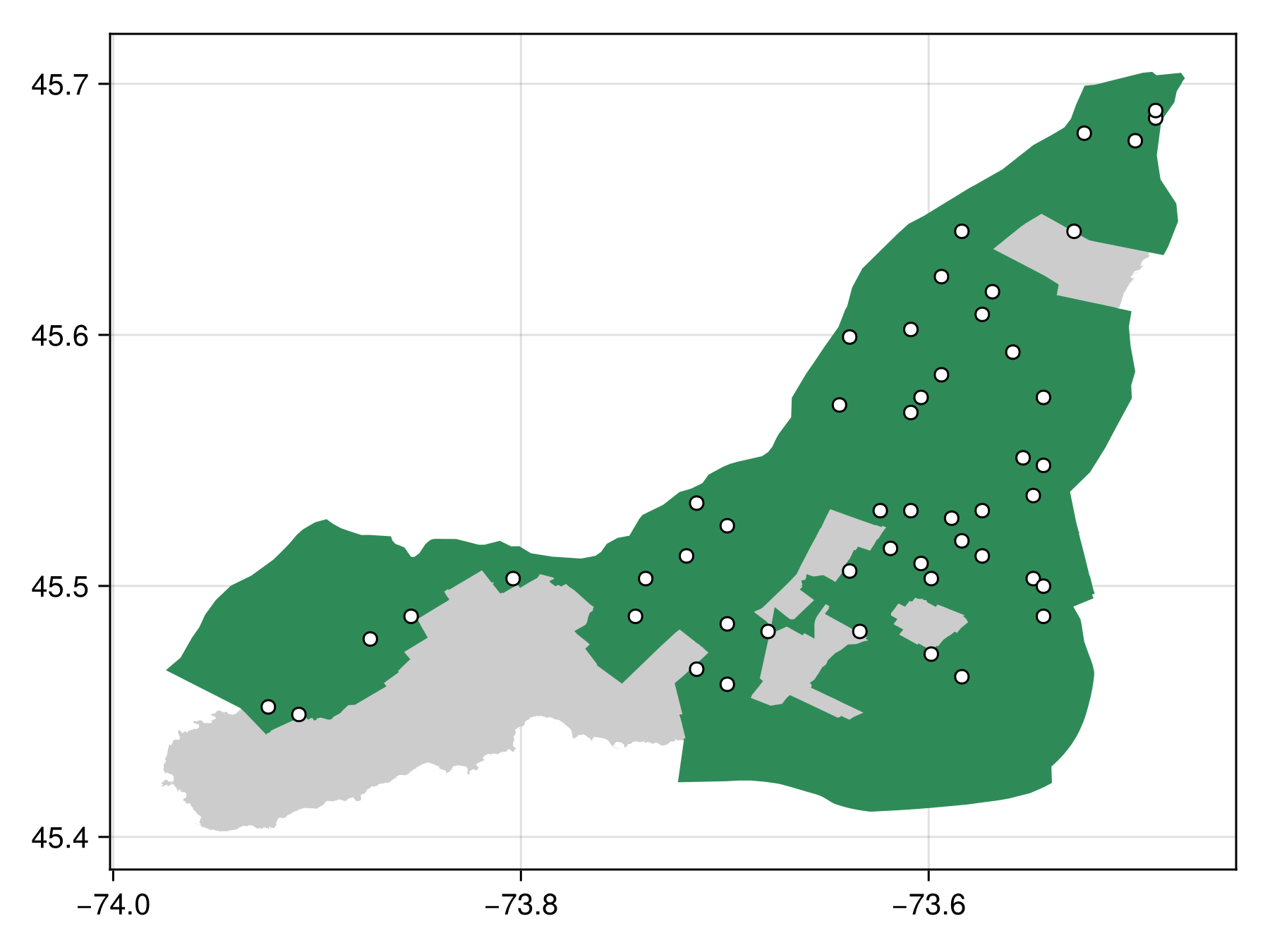
Code for the figure

fig = Figure()
ax = Axis(fig[1,1])
poly!(montreal, color=:grey80)
poly!(ville_de_m, color=:seagreen4)
scatter!(masked_poly_bon, color=:white, strokewidth=1, strokecolor=:black)

Under the hood with polygons

When using a vector-based domain, the vector data is first rasterized because all sampling algorithms work on discrete sets of points.

The size at which they are rasterized is controllable with the resolution keyword argument. By default, it is (100, 100).

We can rasterize at a very coarse resolution to get a better of what's happening

coarse_bon = sample(SimpleRandom(35), montreal; resolution = (10, 10))

BiodiversityObservationNetwork(35 sites via SimpleRandom)

Note at a resolution this coarse, it is possible to see the underlying grid from which the points are selected.

Code for the figure

fig = Figure()
ax = Axis(fig[1,1])
poly!(montreal)
scatter!(coarse_bon, color=:white, strokewidth=1, strokecolor=:black)

Using vector domains with inclusion probabilities

Custom inclusion probabilities can also be used with vector domains, but because vector domains are first rasterized before sampling (as described above), the provided inclusion probabilities must have the same resolution as the rasterized polygon. The easiest way to do this is to pass the resolution keyword argument to sample to ensure the vector domain is rasterized to the same size as the provided inclusions.

Vector domains with matrix inclusion

Using a standard matrix as inclusion is supported. Here we create a 50 x 50 matrix of inclusion that increases toward the right, and then pass the size to the resolution keyword argument to ensure the rasterized vector domain is compatible.

res = (50,50)

inclusion_matrix = [1.2^j for i in 1:res[1], j in 1:res[2]];
inclusion_poly_bon = sample(SimpleRandom(), montreal, inclusion=inclusion_matrix, resolution=size(inclusion_matrix))

BiodiversityObservationNetwork(50 sites via SimpleRandom)

#fig-matrix-inclusion-vec-domain
f = Figure()
ax = Axis(f[1,1])
poly!(ax, montreal)
scatter!(ax, inclusion_poly_bon, color=:white, strokewidth=1, strokecolor=:black)

Vector domains with SDMLayer inclusion

Similarly, an SDMLayer can be used as inclusion probabilities. It is important that the geosptial extent of the SDMLayer overlaps with the vector domain. We do this by explicitly constructing an SDMLayer with the same bounding box as the vector domain:

bbox = SpeciesDistributionToolkit.boundingbox(montreal)
inclusion_matrix = [1.2^j for i in 1:res[1], j in 1:res[2]];
inclusion_layer = SDMLayer(
    inclusion_matrix,
    x = (bbox.left, bbox,right),
    y = (bbox.bottom, bbox.top)
)

🗺️  A 50 × 50 layer with 2500 Float64 cells
   Spatial Reference System: +proj=longlat +datum=WGS84 +no_defs

and sample as BON in a similar way

inclusion_poly_bon = sample(SimpleRandom(), montreal, inclusion=inclusion_layer, resolution=res)

BiodiversityObservationNetwork(50 sites via SimpleRandom)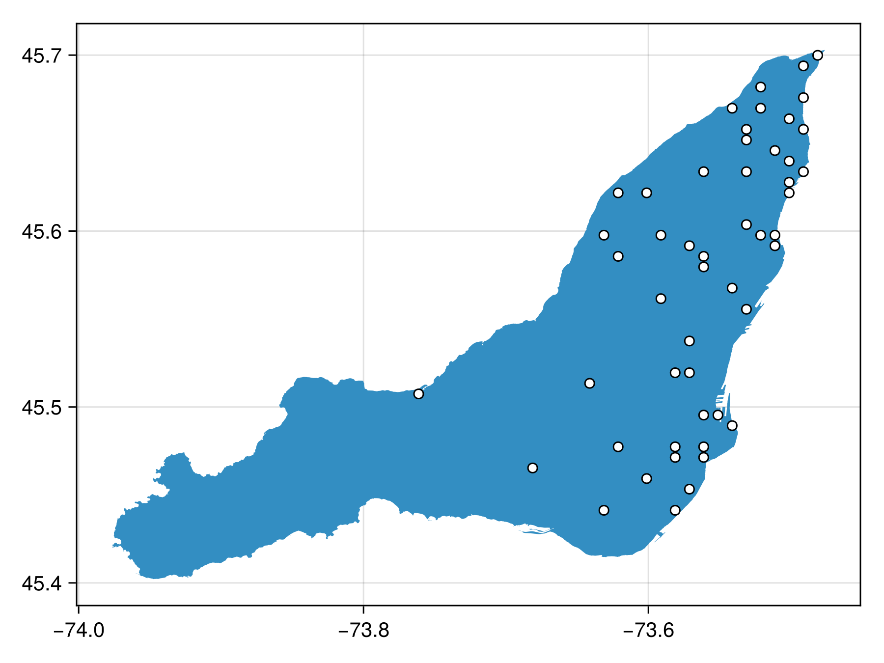

Code for the figure

f = Figure()
ax = Axis(f[1,1])
poly!(ax, montreal)
scatter!(ax, inclusion_poly_bon, color=:white, strokewidth=1, strokecolor=:black)

Next Steps

The next tutorial focuses on using SpeciesDistributionToolkit.jl to prepare climatic geospatial data to target sampling design toward unique climates, or climates expected to change the most in the future.